Using sample representation methods

Using sample representation methods#

In this tutorial, we will demostrate how to use patpy to build sample representation from single-cell transcriptomics data, and how to compare representations from different methods

Install the patpy package#

This package contains interface to sample representation methods as well as some handy analysis functions.

!pip install git+https://github.com/lueckenlab/patpy.git@main

Import packages#

import ehrapy as ep
import pandas as pd
import scanpy as sc
import patpy
import seaborn as sns
from plottable import ColumnDefinition, Table
from plottable.cmap import normed_cmap
from plottable.plots import bar
import matplotlib
import matplotlib.pyplot as plt
from matplotlib.colors import LinearSegmentedColormap

patpy.__version__

'0.9.0'

Read the data#

Here, we use COMBAT dataset. This dataset contains 783k cells from 140 COVID-19 patients and healthy donors.

ADATA_PATH = "/Users/vladimir.shitov/Documents/programming/pat_rep_benchmark/data/combat/combat_processed.h5ad"

adata = sc.read_h5ad(ADATA_PATH)
adata

AnnData object with n_obs × n_vars = 783677 × 3000
    obs: 'Annotation_cluster_id', 'Annotation_cluster_name', 'Annotation_minor_subset', 'Annotation_major_subset', 'Annotation_cell_type', 'GEX_region', 'QC_ngenes', 'QC_total_UMI', 'QC_pct_mitochondrial', 'QC_scrub_doublet_scores', 'TCR_chain_composition', 'TCR_clone_ID', 'TCR_clone_count', 'TCR_clone_proportion', 'TCR_contains_unproductive', 'TCR_doublet', 'TCR_chain_TRA', 'TCR_v_gene_TRA', 'TCR_d_gene_TRA', 'TCR_j_gene_TRA', 'TCR_c_gene_TRA', 'TCR_productive_TRA', 'TCR_cdr3_TRA', 'TCR_umis_TRA', 'TCR_chain_TRA2', 'TCR_v_gene_TRA2', 'TCR_d_gene_TRA2', 'TCR_j_gene_TRA2', 'TCR_c_gene_TRA2', 'TCR_productive_TRA2', 'TCR_cdr3_TRA2', 'TCR_umis_TRA2', 'TCR_chain_TRB', 'TCR_v_gene_TRB', 'TCR_d_gene_TRB', 'TCR_j_gene_TRB', 'TCR_c_gene_TRB', 'TCR_productive_TRB', 'TCR_chain_TRB2', 'TCR_v_gene_TRB2', 'TCR_d_gene_TRB2', 'TCR_j_gene_TRB2', 'TCR_c_gene_TRB2', 'TCR_productive_TRB2', 'TCR_cdr3_TRB2', 'TCR_umis_TRB2', 'BCR_umis_HC', 'BCR_contig_qc_HC', 'BCR_functionality_HC', 'BCR_v_call_HC', 'BCR_v_score_HC', 'BCR_j_call_HC', 'BCR_j_score_HC', 'BCR_junction_aa_HC', 'BCR_total_mut_HC', 'BCR_s_mut_HC', 'BCR_r_mut_HC', 'BCR_c_gene_HC', 'BCR_clone_per_replicate_HC', 'BCR_clone_global_HC', 'BCR_clonal_abundance_HC', 'BCR_locus_LC', 'BCR_umis_LC', 'BCR_contig_qc_LC', 'BCR_functionality_LC', 'BCR_v_call_LC', 'BCR_v_score_LC', 'BCR_j_call_LC', 'BCR_j_score_LC', 'BCR_junction_aa_LC', 'BCR_total_mut_LC', 'BCR_s_mut_LC', 'BCR_r_mut_LC', 'BCR_c_gene_LC', 'COMBAT_ID', 'scRNASeq_sample_ID', 'COMBAT_participant_timepoint_ID', 'Source', 'Age', 'Sex', 'Race', 'BMI', 'Hospitalstay', 'Death28', 'Institute', 'PreExistingHeartDisease', 'PreExistingLungDisease', 'PreExistingKidneyDisease', 'PreExistingDiabetes', 'PreExistingHypertension', 'PreExistingImmunocompromised', 'Smoking', 'Symptomatic', 'Requiredvasoactive', 'Respiratorysupport', 'SARSCoV2PCR', 'Outcome', 'TimeSinceOnset', 'Ethnicity', 'Tissue', 'DiseaseClassification', 'Pool_ID', 'Channel_ID', 'ifn_1_score', '_scvi_batch', '_scvi_labels', 'n_genes_by_counts', 'log1p_n_genes_by_counts', 'total_counts', 'log1p_total_counts', 'pct_counts_in_top_50_genes', 'pct_counts_in_top_100_genes', 'pct_counts_in_top_200_genes', 'pct_counts_in_top_500_genes', 'total_counts_mt', 'log1p_total_counts_mt', 'pct_counts_mt', 'total_counts_ribo', 'log1p_total_counts_ribo', 'pct_counts_ribo'
    var: 'gene_ids', 'feature_types', 'highly_variable', 'highly_variable_rank', 'means', 'variances', 'variances_norm', 'highly_variable_nbatches', 'mt', 'ribo', 'n_cells_by_counts', 'mean_counts', 'log1p_mean_counts', 'pct_dropout_by_counts', 'total_counts', 'log1p_total_counts'
    uns: 'Institute', 'ObjectCreateDate', 'Source_colors', 'Technology', 'X_scpoli', '_scvi_manager_uuid', '_scvi_uuid', 'genome_annotation_version', 'hvg', 'log1p', 'pca', 'scpoli_distances', 'scpoli_parameters', 'scpoli_samples'
    obsm: 'X_pca', 'X_scANVI_batch', 'X_scANVI_sample', 'X_scVI_batch', 'X_scVI_sample', 'X_scpoli', 'X_umap', 'X_umap_source'
    varm: 'PCs'
    layers: 'X_raw_counts'

Set columns containing sample IDs, cell types and metadata#

sample_id_col = "scRNASeq_sample_ID"
cell_type_key = "cell_type"
samples_metadata_cols = ["Source", "Outcome", "Death28", "Institute", "Pool_ID"]

Currently, there is no such columns as “cell_type” in the data. But cell types are stored in the Annotation_major_subset column. Let’s rename it to cell_type for better readability.

adata.obs.rename(columns={"Annotation_major_subset": cell_type_key}, inplace=True)

Store metadata and calculate QC metrics#

metadata = adata.obs[samples_metadata_cols + [sample_id_col]].drop_duplicates()
metadata.set_index(sample_id_col, inplace=True)
metadata

	Source	Outcome	Death28	Institute	Pool_ID
scRNASeq_sample_ID
S00109-Ja001E-PBCa	COVID_SEV	2.0	0	Oxford	gPlexA
S00112-Ja003E-PBCa	COVID_MILD	5.0	0	Oxford	gPlexA
S00005-Ja005E-PBCa	COVID_CRIT	2.0	0	Oxford	gPlexA
S00061-Ja003E-PBCa	COVID_SEV	4.0	0	Oxford	gPlexA
S00056-Ja003E-PBCa	COVID_SEV	3.0	0	Oxford	gPlexA
...	...	...	...	...	...
S00065-Ja003E-PBCa	COVID_CRIT	2.0	0	Oxford	gPlexK
S00048-Ja003E-PBCa	COVID_SEV	4.0	0	Oxford	gPlexK
G05112-Ja005E-PBCa	COVID_HCW_MILD	6.0	0	Oxford	gPlexK
N00038-Ja001E-PBGa	Sepsis	NaN	0	Oxford	gPlexK
U00501-Ua005E-PBUa	Flu	2.0	0	St_Georges	gPlexK

138 rows × 5 columns

cell_qc_metadata = patpy.pp.calculate_cell_qc_metrics(
    adata, sample_key=sample_id_col, cell_qc_vars=["QC_ngenes", "QC_pct_mitochondrial", "QC_scrub_doublet_scores"]
)
cell_qc_metadata

	median_QC_ngenes	median_QC_pct_mitochondrial	median_QC_scrub_doublet_scores
scRNASeq_sample_ID
G05061-Ja005E-PBCa	1107.0	3.011159	0.050648
G05064-Ja005E-PBCa	975.0	1.332430	0.060894
G05073-Ja005E-PBCa	1141.0	2.422559	0.044530
G05077-Ja005E-PBCa	1125.0	2.946723	0.048490
G05078-Ja005E-PBCa	999.0	2.825308	0.052783
...	...	...	...
U00607-Ua005E-PBUa	1827.0	2.982509	0.043323
U00613-Ua005E-PBUa	1251.5	2.053083	0.036956
U00617-Ua005E-PBUa	1410.5	3.886215	0.057906
U00619-Ua005E-PBUa	1532.0	2.688350	0.041823
U00701-Ua005E-PBUa	1093.5	3.714650	0.063941

138 rows × 3 columns

n_genes_metadata = patpy.pp.calculate_n_cells_per_sample(adata, sample_id_col)
n_genes_metadata

	n_cells
scRNASeq_sample_ID
S00052-Ja005E-PBCa	13918
H00054-Ha001E-PBGa	10938
H00067-Ha001E-PBGa	10781
N00023-Ja001E-PBGa	10484
H00053-Ha001E-PBGa	10458
...	...
U00607-Ua005E-PBUa	1021
U00613-Ua005E-PBUa	970
U00701-Ua005E-PBUa	872
U00601-Ua005E-PBUa	619
U00504-Ua005E-PBUa	161

138 rows × 1 columns

composition_metadata = patpy.pp.calculate_compositional_metrics(adata, sample_id_col, [cell_type_key], normalize_to=100)
composition_metadata

cell_type	cell_type_B	cell_type_CD4	cell_type_CD8	cell_type_DC	cell_type_DN	cell_type_DP	cell_type_GDT	cell_type_HSC	cell_type_MAIT	cell_type_Mast	cell_type_NK	cell_type_PB	cell_type_PLT	cell_type_RET	cell_type_cMono	cell_type_iNKT	cell_type_ncMono
scRNASeq_sample_ID
G05061-Ja005E-PBCa	6.324900	33.921438	12.366844	1.597870	0.532623	0.499334	0.898802	0.066578	4.677097	0.000000	18.159121	0.316245	0.166445	0.016644	15.812250	0.033289	4.610519
G05064-Ja005E-PBCa	3.405158	47.147482	16.400581	1.819806	1.228090	0.725689	2.188233	0.022329	1.317405	0.000000	7.457854	0.446578	0.000000	0.000000	14.357486	0.000000	3.483309
G05073-Ja005E-PBCa	5.194338	45.609405	16.278791	1.487524	1.247601	0.839731	4.654511	0.011996	2.195298	0.011996	3.730806	0.203935	0.047985	0.000000	13.963532	0.083973	4.438580
G05077-Ja005E-PBCa	5.846211	29.231056	14.596909	1.377770	0.446844	1.340532	0.465463	0.167567	0.800596	0.018619	22.844908	1.079873	0.074474	0.018619	18.004096	0.055856	3.630609
G05078-Ja005E-PBCa	1.366381	39.000106	15.591569	2.340854	0.762631	0.730855	2.648025	0.211842	1.737104	0.021184	10.666243	0.148289	0.021184	0.000000	19.521237	0.497829	4.734668
...	...	...	...	...	...	...	...	...	...	...	...	...	...	...	...	...	...
U00607-Ua005E-PBUa	3.623898	10.577865	1.273262	4.701273	0.097943	0.195886	0.195886	0.685602	0.097943	0.000000	5.876592	1.175318	1.958864	0.097943	37.904016	0.000000	31.537708
U00613-Ua005E-PBUa	7.835052	26.391753	16.907216	0.721649	0.412371	0.309278	1.649485	0.000000	0.103093	0.000000	5.154639	1.237113	0.206186	0.000000	37.938144	0.000000	1.134021
U00617-Ua005E-PBUa	2.977233	41.418564	16.462347	0.437828	0.525394	0.262697	0.262697	0.963222	0.087566	0.000000	7.530648	17.513135	0.788091	0.087566	9.719790	0.000000	0.963222
U00619-Ua005E-PBUa	3.537618	35.077230	15.894370	0.896861	0.697559	0.298954	2.441455	1.145989	0.099651	0.099651	17.588440	2.840060	4.534131	0.000000	10.363727	0.000000	4.484305
U00701-Ua005E-PBUa	1.032110	15.596330	39.334862	1.261468	0.802752	0.458716	0.573394	0.114679	0.000000	0.000000	12.844037	0.000000	0.344037	0.229358	24.885321	0.000000	2.522936

138 rows × 17 columns

Merge metadata tables

metadata = pd.concat(
    [
        metadata,
        cell_qc_metadata.loc[metadata.index],
        n_genes_metadata.loc[metadata.index],
        composition_metadata.loc[metadata.index],
    ],
    axis=1,
)

metadata.shape

../_images/3c6e42d2351a31b9ea880c4957a4cdd76cf57e4348c2ebacc9f9caad4353d0a4.png

Quality control#

To reduce noise in the representations, we need to remove samples with too few cells:

adata = patpy.pp.filter_small_samples(adata, sample_key=sample_id_col, sample_size_threshold=100)

0 samples removed:

If necessary, we can also remove cell types with too few cells in at least one sample:

adata = patpy.pp.filter_small_cell_types(adata, sample_key=sample_id_col, cell_group_key=cell_type_key, cell_type_size_threshold=10)

Some methods require this filtering step prior to building representation. In this notebook, we’ll focus on simpler methods that can be used with only sample filtering.

Run a simple pseudobulk representation#

This method aggregates all cells from each sample into a single vector. It can be interpreted as an average cell from each sample. Any input space can be used specified by layer parameter. For example, to use count data, use layer="X" or layer="raw". We find batch-corrected space to be the best for the representation, so we use layer="X_scVI" below.

pseudobulk = patpy.tl.Pseudobulk(sample_key=sample_id_col, cell_group_key=cell_type_key, layer="X_scVI_batch")
pseudobulk.prepare_anndata(adata)

Calculate a matrix of distances between samples#

distances = pseudobulk.calculate_distance_matrix(force=True)
distances

array([[0.        , 2.13826083, 3.26751086, ..., 2.26537604, 3.47556017,
        3.50837059],
       [2.13826083, 0.        , 2.57066436, ..., 2.67332482, 3.12726692,
        2.3833747 ],
       [3.26751086, 2.57066436, 0.        , ..., 3.81414183, 3.50147504,
        2.11261287],
       ...,
       [2.26537604, 2.67332482, 3.81414183, ..., 0.        , 3.55756191,
        4.0558818 ],
       [3.47556017, 3.12726692, 3.50147504, ..., 3.55756191, 0.        ,
        2.70576771],
       [3.50837059, 2.3833747 , 2.11261287, ..., 4.0558818 , 2.70576771,
        0.        ]])

We can also see the pseudobulks for each sample:

pseudobulk.sample_representation

array([[-0.39708972, -0.1610353 , -0.60592145, ...,  0.04138801,
        -0.23706943,  0.03939089],
       [-0.16564418,  0.15338482, -0.00623349, ..., -0.36909145,
        -0.61890358, -0.26146826],
       [-0.91906726, -0.34432968, -0.03022187, ..., -1.03792512,
        -0.26926878,  0.30427763],
       ...,
       [ 0.07143331, -0.52035475, -0.04083514, ..., -0.01975986,
        -0.2641018 , -0.32993519],
       [-0.86681354, -0.71001476,  0.40946293, ...,  0.38672951,
         0.59467804,  0.03230282],
       [-0.98729014, -0.46418488,  0.28515279, ..., -0.19687848,
        -0.42034405,  0.18162856]])

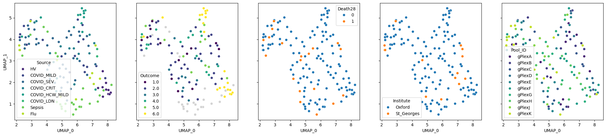
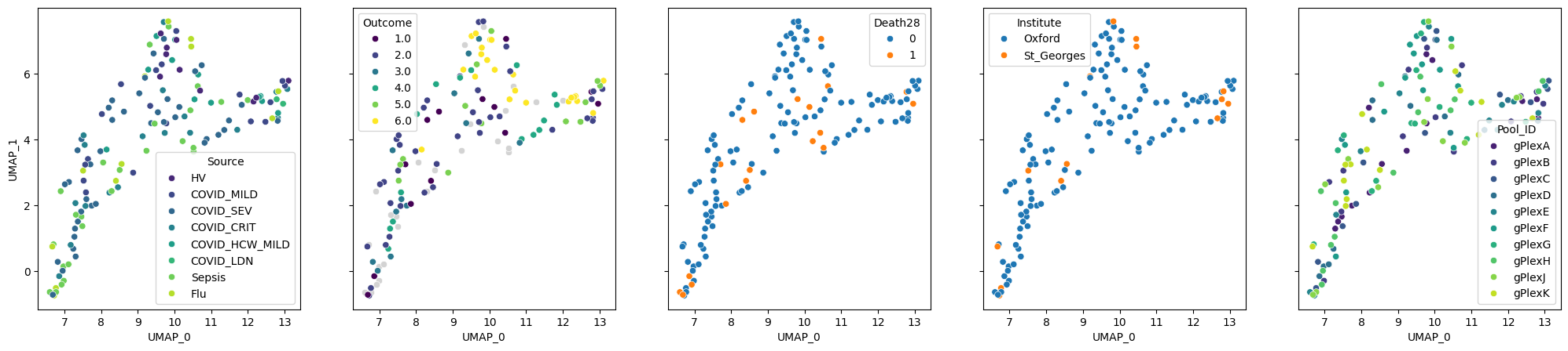
We can then visualise sample representation using dimensionality reduction methods:

pseudobulk.plot_embedding(method="UMAP", metadata_cols=samples_metadata_cols);

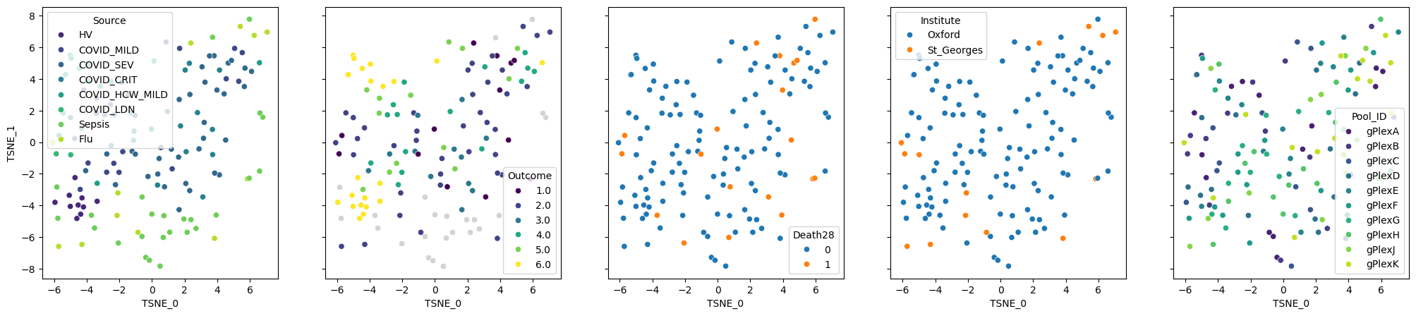
../_images/28cd87a22835b3681eeb09461f573aeea1623536cff4a8882dff04a18d66a122.png

Other dimensionality reduction methods are also available

pseudobulk.plot_embedding(method="TSNE", metadata_cols=samples_metadata_cols);

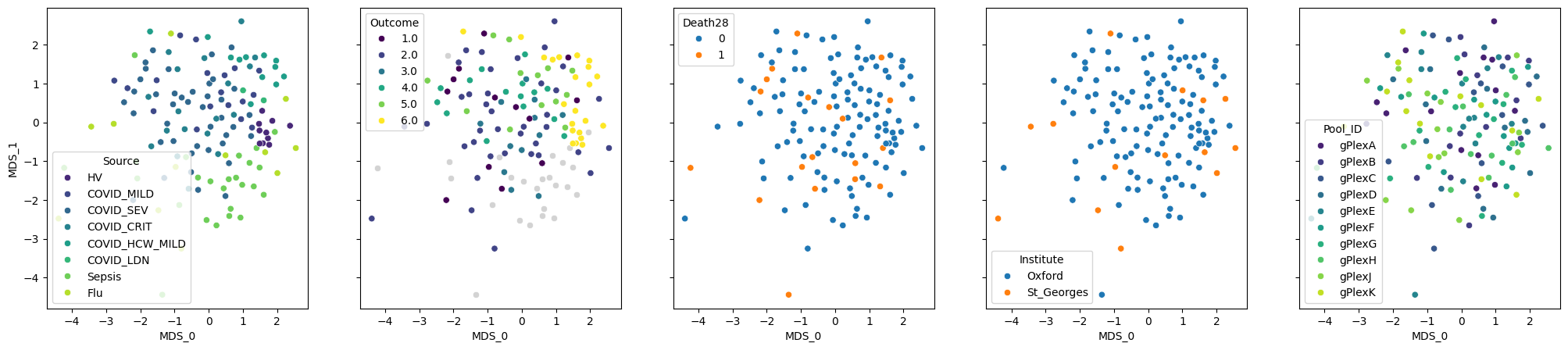
../_images/8e9158dc7ba1b1c8df50b9d4cb6ce45dd8796d1068c43e2493151ba9b16dd1ec.png

pseudobulk.plot_embedding(method="MDS", metadata_cols=samples_metadata_cols);

../_images/066a51f3f96d167305e60a437d8ee6ebcd05c63aadb4d55232aeb2774618351c.png

Evaluate how well a covariate is represented#

Let’s try to classify “Outcome” based on the nearest neighbors for each sample in the representation:

pseudobulk.evaluate_representation(target="Outcome", method="knn", n_neighbors=5, task="classification")

{'score': 0.13977126662840952,
 'metric': 'f1_macro_calibrated',
 'n_unique': 6,
 'n_observations': 113,
 'method': 'knn'}

It doesn’t work too good. Now we can try to solve the ranking problem for the same covariate. It will train regressor and use a different metric for evaluation:

pseudobulk.evaluate_representation(target="Outcome", method="knn", n_neighbors=5, task="ranking")

{'score': 0.6103813851943187,
 'metric': 'spearman_r',
 'n_unique': 6,
 'n_observations': 113,
 'method': 'knn'}

Now let’s see how well Pool is represented. This is a technical covariate so we don’t want score to be high:

pseudobulk.evaluate_representation(target="Pool_ID", method="knn", n_neighbors=5, task="classification")

{'score': 0.13579292359838518,
 'metric': 'f1_macro_calibrated',
 'n_unique': 10,
 'n_observations': 138,
 'method': 'knn'}

Save the distances to adata to use later

adata.uns["pseudobulk_distances"] = distances
adata.uns["pseudobulk_samples"] = pseudobulk.samples
adata.uns["pseudobulk_UMAP"] = pseudobulk.embeddings["UMAP"]

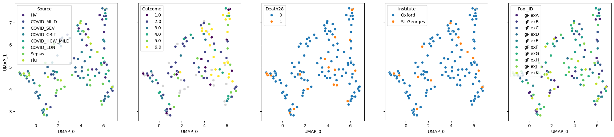
Run cell type composition representation#

This representation is based on cell type composition differences. It is calculated as a difference between cell type proportions in each sample.

composition = patpy.tl.CellGroupComposition(sample_key=sample_id_col, cell_group_key=cell_type_key, layer="X_scVI")
composition.prepare_anndata(adata)
composition_distances = composition.calculate_distance_matrix(force=True)

composition.plot_embedding(method="UMAP", metadata_cols=samples_metadata_cols)

array([<Axes: xlabel='UMAP_0', ylabel='UMAP_1'>,
       <Axes: xlabel='UMAP_0', ylabel='UMAP_1'>,
       <Axes: xlabel='UMAP_0', ylabel='UMAP_1'>,
       <Axes: xlabel='UMAP_0', ylabel='UMAP_1'>,
       <Axes: xlabel='UMAP_0', ylabel='UMAP_1'>], dtype=object)

../_images/32bf43eca2ff933e03f3e38ca4d3c433af41e4e7bfcd1c842247fd6b552e21d2.png

We can also visualise cell type proportions for each sample:

composition.sample_representation.plot(kind="bar", stacked=True, figsize=(10, 8), width=0.8)
plt.xticks([])
plt.legend(loc=(1.05, 0), title="Cell type");

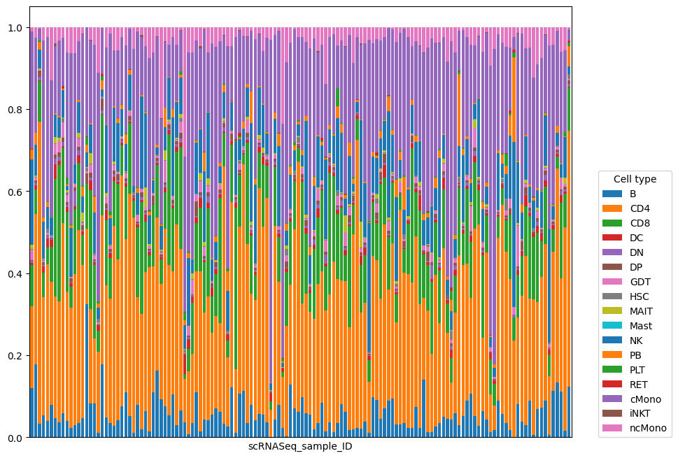
../_images/da85b264f2f02e1e83adab7141d11c306e6495e14f1f2bc030aaf8b6a61991d6.png

We can see that cell type composition reflects patient outcome worse than pseudobulk:

composition.evaluate_representation(target="Outcome", method="knn", n_neighbors=5, task="ranking")

{'score': 0.4739538892493282,
 'metric': 'spearman_r',
 'n_unique': 6,
 'n_observations': 113,
 'method': 'knn'}

adata.uns["composition_distances"] = composition_distances
adata.uns["composition_samples"] = composition.samples

Run PILOT representation#

PILOT is an Optimal Transport-based tool, which calculates distances between samples based on cell type proportion differences taking into account cell type similarities. Note that to run it, you need to install the dependencies additionally:

pip install patpy[pilot]

pilot = patpy.tl.PILOT(
    sample_key=sample_id_col,
    cell_group_key=cell_type_key,
    layer="X_scVI_batch",
    sample_state_col="Outcome",  # It is not used for distances calculation and doesn't really matter
)

pilot.prepare_anndata(adata)

pilot.calculate_distance_matrix()

array([[0.        , 0.14451829, 0.42457524, ..., 0.10953257, 0.21343671,
        0.36804272],
       [0.14451829, 0.        , 0.32280757, ..., 0.10045083, 0.13157015,
        0.25766875],
       [0.42457524, 0.32280757, 0.        , ..., 0.36857701, 0.23438838,
        0.08670158],
       ...,
       [0.10953257, 0.10045083, 0.36857701, ..., 0.        , 0.17271665,
        0.31134621],
       [0.21343671, 0.13157015, 0.23438838, ..., 0.17271665, 0.        ,
        0.21202688],
       [0.36804272, 0.25766875, 0.08670158, ..., 0.31134621, 0.21202688,
        0.        ]])

pilot.plot_embedding(method="UMAP", metadata_cols=samples_metadata_cols);

../_images/d69cd8503effd2414a8558a27b7ae298c7676cf64bb9826191e3d5bce4cca615.png

adata.uns["pilot_distances"] = pilot.calculate_distance_matrix()
adata.uns["pilot_samples"] = pilot.samples
adata.uns["pilot_UMAP"] = pilot.embeddings["UMAP"]

Let’s check the covariates:

pilot.evaluate_representation(target="Outcome", method="knn", n_neighbors=5, task="ranking")

{'score': 0.48835133146990367,
 'metric': 'spearman_r',
 'n_unique': 6,
 'n_observations': 113,
 'method': 'knn'}

pilot.evaluate_representation(target="Pool_ID", method="knn", n_neighbors=5, task="classification")

{'score': 0.01832203003010072,
 'metric': 'f1_macro_calibrated',
 'n_unique': 10,
 'n_observations': 138,
 'method': 'knn'}

Outcome is represented a bit worse, but Pool ID almost doesn’t affect the representation

Compare representations#

Let’s write a small function to put all the sample representations into a single object. It will make sure that the order of samples is identical and cluster the patients

def align_representations(adata, meta_adata, samples, methods):
    """
    Align representations of different methods to have the same order of samples.

    Additionally runs clustering with Leiden algorithm.
    """
    for method in methods:
        #     samples_to_take = np.isin(adata.uns[f"{method}_samples"], samples)
        representation_samples = adata.uns[f"{method}_samples"].tolist()
        samples_order = [representation_samples.index(sample) for sample in samples if sample in representation_samples]

        assert (adata.uns[f"{method}_samples"][samples_order] == samples).all(), "Order of samples is not correct"

        # meta_adata.obsm["umap"] = meta_adata.obsm[f"{method}_UMAP"]
        meta_adata.obsm[f"{method}_distances"] = adata.uns[f"{method}_distances"][samples_order][:, samples_order]

        ep.pp.neighbors(
            meta_adata, use_rep=f"{method}_distances", key_added=f"{method}_neighbors", metric="precomputed"
        )
        ep.tl.leiden(meta_adata, key_added=f"{method}_leiden", neighbors_key=f"{method}_neighbors")

    return meta_adata

combat_methods = [
    "pseudobulk",
    "composition",
    "pilot",
]

combat_samples = list(set(adata.uns[f"{method}_samples"]) for method in combat_methods)
combat_samples = list(set.intersection(*combat_samples))
len(combat_samples)

../_images/b3437138c30d612d3e297c9ce3829756b344b4a0cb5f4ce5e8f0633222774fc7.png

metadata = metadata.loc[combat_samples]

combat_meta_adata = ep.io.df_to_anndata(metadata)
combat_meta_adata = ep.pp.encode(combat_meta_adata, autodetect=True)
combat_meta_adata

! Features 'Outcome', 'Death28' were detected as categorical features stored numerically.Please verify and correct using `ep.ad.replace_feature_types` if necessary.
! Feature types were inferred and stored in adata.var[feature_type]. Please verify using `ep.ad.feature_type_overview` and adjust if necessary using `ep.ad.replace_feature_types`.

AnnData object with n_obs × n_vars = 138 × 43
    obs: 'Source', 'Institute', 'Pool_ID'
    var: 'feature_type', 'unencoded_var_names', 'encoding_mode'
    layers: 'original'

combat_meta_adata = align_representations(
    adata=adata,
    meta_adata=combat_meta_adata,
    samples=combat_samples,
    methods=combat_methods,
)

Define types and prediction tasks for the covariates#

benchmark_schema = {
    "technical": ["Institute", "Pool_ID", "n_cells", "median_QC_ngenes"],
    "clinical": ["Death28", "Outcome", "Source"],
}

cols_with_tasks = {
    "Institute": "classification",
    "Pool_ID": "classification",
    "n_cells": "regression",
    "median_QC_ngenes": "regression",
    "Death28": "classification",
    "Outcome": "ranking",
    "Source": "classification",
}

results = []

for method in combat_methods:
    for covariate_type in benchmark_schema:
        for col in benchmark_schema[covariate_type]:
            task = cols_with_tasks[col]
            try:
                result = patpy.tl.evaluate_representation(
                    distances=combat_meta_adata.obsm[f"{method}_distances"],
                    target=metadata[col],
                    method="knn",
                    task=task,
                    #             n_neighbors=5
                )
            except Exception as e:
                print("Method:", method)
                print("Col:", col)
                print("Task:", task)
                print(e)
                print()
                continue
            #             raise(e)
            result["representation"] = method
            result["covariate"] = col
            result["covariate_type"] = covariate_type

            if result["metric"] == "spearman_r":
                result["score"] = abs(result["score"])

            if covariate_type == "technical":
                result["score"] = 1 - result["score"]

            results.append(result)

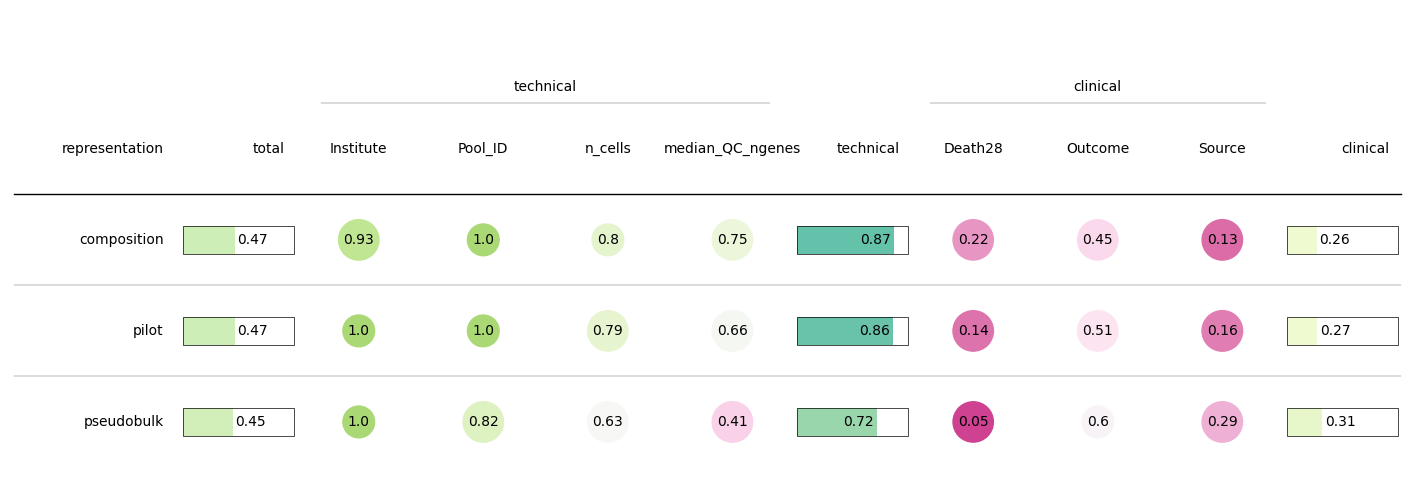
Scores are ranged from 0 to 1

For covariates that we defined as technical, 0 means that covariate strongly affects the representation, and 1 means that this covariate is randomly distributed across representation
For biological and clinical covariates, 0 means that a covariate is not represented well (it is randomly distributed), while 1 means that similar patients have similar values of covariate

knn_results = pd.DataFrame(results)
knn_results.sort_values("score", ascending=False)

	score	metric	n_unique	n_observations	method	representation	covariate	covariate_type
0	1.000000	f1_macro_calibrated	2	138	knn	pseudobulk	Institute	technical
8	1.000000	f1_macro_calibrated	10	138	knn	composition	Pool_ID	technical
15	1.000000	f1_macro_calibrated	10	138	knn	pilot	Pool_ID	technical
14	1.000000	f1_macro_calibrated	2	138	knn	pilot	Institute	technical
7	0.928846	f1_macro_calibrated	2	138	knn	composition	Institute	technical
1	0.824655	f1_macro_calibrated	10	138	knn	pseudobulk	Pool_ID	technical
9	0.803490	spearman_r	138	138	knn	composition	n_cells	technical
16	0.792614	spearman_r	138	138	knn	pilot	n_cells	technical
10	0.752516	spearman_r	119	138	knn	composition	median_QC_ngenes	technical
17	0.656404	spearman_r	119	138	knn	pilot	median_QC_ngenes	technical
2	0.632495	spearman_r	138	138	knn	pseudobulk	n_cells	technical
5	0.603334	spearman_r	6	113	knn	pseudobulk	Outcome	clinical
19	0.505120	spearman_r	6	113	knn	pilot	Outcome	clinical
12	0.446273	spearman_r	6	113	knn	composition	Outcome	clinical
3	0.414135	spearman_r	119	138	knn	pseudobulk	median_QC_ngenes	technical
6	0.292073	f1_macro_calibrated	8	138	knn	pseudobulk	Source	clinical
11	0.219991	f1_macro_calibrated	2	138	knn	composition	Death28	clinical
20	0.160770	f1_macro_calibrated	8	138	knn	pilot	Source	clinical
18	0.137885	f1_macro_calibrated	2	138	knn	pilot	Death28	clinical
13	0.125450	f1_macro_calibrated	8	138	knn	composition	Source	clinical
4	0.046083	f1_macro_calibrated	2	138	knn	pseudobulk	Death28	clinical

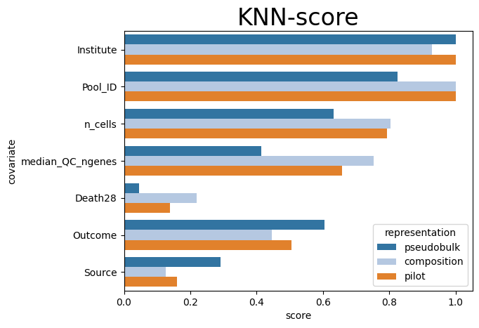
# plt.figure(figsize=(10, 20))
sns.barplot(data=knn_results, y="covariate", x="score", orient="h", hue="representation", palette="tab20")
plt.xlim(0, 1.05)
plt.title("KNN-score", fontsize=24)

Text(0.5, 1.0, 'KNN-score')

../_images/259f807ab05daf35573f1c776bbd07b407a4009cfa6b95455b8a212766e05cdf.png

knn_results_wide = knn_results.pivot(index="representation", columns="covariate", values="score")
# knn_results_wide.reset_index(inplace=True)

# Order the columns as in benchmark schema
cols_order = ["total"]

for covariate_type in benchmark_schema:
    cols_order.extend(benchmark_schema[covariate_type])
    cols_order.append(covariate_type)

cmap = LinearSegmentedColormap.from_list(
    name="bugw", colors=["#FF9693", "#f2fbd2", "#c9ecb4", "#93d3ab", "#35b0ab"], N=256
)

col_defs = []

col_defs.append(
    ColumnDefinition(
        "total",
        width=0.7,
        plot_fn=bar,
        plot_kw={
            "cmap": cmap,
            "plot_bg_bar": True,
            "annotate": True,
            "height": 0.5,
            "lw": 0.5,
            "formatter": lambda x: round(x, 2),
        },
    )
)

for covariate_type in benchmark_schema:
    type_cols = benchmark_schema[covariate_type]

    for col in type_cols:
        col_def = ColumnDefinition(
            name=col,
            width=0.75,
            formatter=lambda x: round(x, 2),
            textprops={
                "ha": "center",
                "bbox": {"boxstyle": "circle", "pad": 0.35},
            },
            cmap=normed_cmap(knn_results["score"], cmap=matplotlib.cm.PiYG, num_stds=2.5),
            group=covariate_type,
        )

        col_defs.append(col_def)

    knn_results_wide[covariate_type] = knn_results_wide[type_cols].mean(axis=1)
    col_defs.append(
        ColumnDefinition(
            covariate_type,
            width=0.7,
            plot_fn=bar,
            plot_kw={
                "cmap": cmap,
                "plot_bg_bar": True,
                "annotate": True,
                "height": 0.5,
                "lw": 0.5,
                "formatter": lambda x: round(x, 2),
            },
        )
    )


#     col_defs.append(type_cols)
clin_weight = 2 / 3

knn_results_wide["total"] = (
    clin_weight * knn_results_wide["clinical"] + (1 - clin_weight) * knn_results_wide["technical"]
)

fig, ax = plt.subplots(figsize=(18, 6))

Table(knn_results_wide[cols_order].sort_values("total", ascending=False), column_definitions=tuple(col_defs), ax=ax)

<plottable.table.Table at 0x42cf8fd50>

../_images/28516ae9a73375ffeb3c5b5ca30cbf3a034c43adb0e8abf00e5f2429921a773d.png

Other methods#

There are other methods implemented that you might want to try:

Aggregated per cell type (or some other group) pseudobulk: patpy.tl.GroupedPseudobulk
Composition differences: patpy.tl.CellGroupComposition
scPoli: patpy.tl.SCPoli
MrVI: patpy.tl.MrVI
PhEMD: patpy.tl.PhEMD
MOFA: patpy.tl.MOFA
GloScope: patpy.tl.GloScope

In the sample representation benchmark, we found GloScope to be the best representation method. For running it, R installation is required. You can use environment from this repository or manually install required dependencies.