Benchmarking sample representation methods with patpy

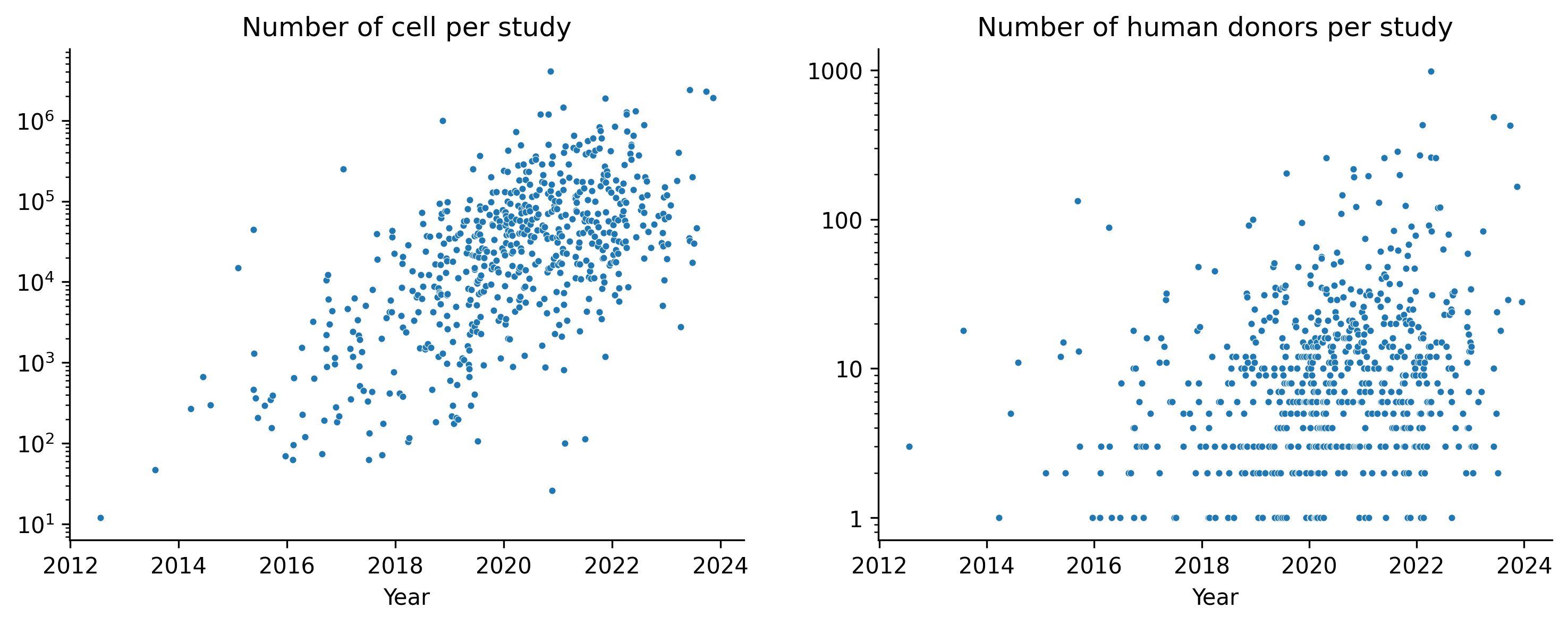
Single-cell transcriptomics provides extremely high resolution view on biology. But many processes, such as diseases or ageing, manifest on tissue or organism level. To understand them, we need to understand diversity on a patient (or donor) level. Single-cell transcriptomics field is therefore moving to generating massive multi-donor datasets and integrated atlasses, containing hundreds to thousands donors per study (Hrovatin, Sikkema, et al, Nature Methods 2025)

Recently, sample (a.k.a. patient or donor) representation methods emerged to explore diversity on donor-level. But which of them work the best? In this tutorial, we’ll show how to use patpy to run and compare different sample representation methods from single-cell data. To see more on benchmarking, refer to our benchmarking preprint Shitov et al, Learning Meaningful Representations of Life (LMRL) Workshop at ICLR 2025

Installation

Before running the code below, make sure you have dependencies installed. Most of what we use ships with the base install (pip install patpy). The deep methods need extras (and ideally a CUDA GPU):

pip install patpy[pilot,mrvi,scpoli,diffusionemd]  # Optional for running deep learning methods
pip install mofapy2  # For running MOFA

Note that installing everything into one enviroment can be challenging. This is especially the case for deep learning methods. For larger-scale benchmarking, we recommend creating method-specific environments

Import packages

import ehrapy as ep  # Like scanpy, but for clinical data analysis. Convenient to preprocess the sample-level data
import scanpy as sc
import patpy  # Datasets, metrics, and analysis of sample representations
import os  # For reading environment variables (e.g. PATPY_GLOSCOPE_GPU)
import pandas as pd  # Working with data frames

# Plotting
import matplotlib
import matplotlib.pyplot as plt
from matplotlib.colors import LinearSegmentedColormap
import seaborn as sns

# For displaying benchmarking metrics
from plottable import ColumnDefinition, Table
from plottable.cmap import normed_cmap
from plottable.plots import bar

import time as _time  # For measuring runtime of the methods

# Use a higher figure DPI for crisper plots in the rendered notebook,
# and remove the top/right spines from any seaborn scatter/bar plots.
matplotlib.rcParams['figure.dpi'] = 150
matplotlib.rcParams['savefig.dpi'] = 150

patpy.__version__

'0.16.5'

Hallmarks of COVID-19 disease severity

We’ll first dive deeply into the COMBAT dataset analysis (COvid-19 Multi-omics Blood ATlas (COMBAT) Consortium, Cell, 2022). This dataset contains 783k peripheral blood mononuclear cells (PBMC) from 140 samples obtained from COVID-19, Flu, and Sepsis patients as well as from healthy donors. This dataset is a perfect sandbox for sample representation methods because it does not suffer from batch effects and hides a very clear COVID-19 severity trajectory. Let’s see which method can uncover it the best.

patpy provides easy access to COMBAT dataset (as well as some others):

adata, adata_info = patpy.datasets.combat(return_dataset_info=True)
adata

AnnData object with n_obs × n_vars = 783677 × 3000
    obs: 'Annotation_cluster_id', 'Annotation_cluster_name', 'Annotation_minor_subset', 'Annotation_major_subset', 'Annotation_cell_type', 'GEX_region', 'QC_ngenes', 'QC_total_UMI', 'QC_pct_mitochondrial', 'QC_scrub_doublet_scores', 'TCR_chain_composition', 'TCR_clone_ID', 'TCR_clone_count', 'TCR_clone_proportion', 'TCR_contains_unproductive', 'TCR_doublet', 'TCR_chain_TRA', 'TCR_v_gene_TRA', 'TCR_d_gene_TRA', 'TCR_j_gene_TRA', 'TCR_c_gene_TRA', 'TCR_productive_TRA', 'TCR_cdr3_TRA', 'TCR_umis_TRA', 'TCR_chain_TRA2', 'TCR_v_gene_TRA2', 'TCR_d_gene_TRA2', 'TCR_j_gene_TRA2', 'TCR_c_gene_TRA2', 'TCR_productive_TRA2', 'TCR_cdr3_TRA2', 'TCR_umis_TRA2', 'TCR_chain_TRB', 'TCR_v_gene_TRB', 'TCR_d_gene_TRB', 'TCR_j_gene_TRB', 'TCR_c_gene_TRB', 'TCR_productive_TRB', 'TCR_chain_TRB2', 'TCR_v_gene_TRB2', 'TCR_d_gene_TRB2', 'TCR_j_gene_TRB2', 'TCR_c_gene_TRB2', 'TCR_productive_TRB2', 'TCR_cdr3_TRB2', 'TCR_umis_TRB2', 'BCR_umis_HC', 'BCR_contig_qc_HC', 'BCR_functionality_HC', 'BCR_v_call_HC', 'BCR_v_score_HC', 'BCR_j_call_HC', 'BCR_j_score_HC', 'BCR_junction_aa_HC', 'BCR_total_mut_HC', 'BCR_s_mut_HC', 'BCR_r_mut_HC', 'BCR_c_gene_HC', 'BCR_clone_per_replicate_HC', 'BCR_clone_global_HC', 'BCR_clonal_abundance_HC', 'BCR_locus_LC', 'BCR_umis_LC', 'BCR_contig_qc_LC', 'BCR_functionality_LC', 'BCR_v_call_LC', 'BCR_v_score_LC', 'BCR_j_call_LC', 'BCR_j_score_LC', 'BCR_junction_aa_LC', 'BCR_total_mut_LC', 'BCR_s_mut_LC', 'BCR_r_mut_LC', 'BCR_c_gene_LC', 'COMBAT_ID', 'scRNASeq_sample_ID', 'COMBAT_participant_timepoint_ID', 'Source', 'Age', 'Sex', 'Race', 'BMI', 'Hospitalstay', 'Death28', 'Institute', 'PreExistingHeartDisease', 'PreExistingLungDisease', 'PreExistingKidneyDisease', 'PreExistingDiabetes', 'PreExistingHypertension', 'PreExistingImmunocompromised', 'Smoking', 'Symptomatic', 'Requiredvasoactive', 'Respiratorysupport', 'SARSCoV2PCR', 'Outcome', 'TimeSinceOnset', 'Ethnicity', 'Tissue', 'DiseaseClassification', 'Pool_ID', 'Channel_ID', 'ifn_1_score', '_scvi_batch', '_scvi_labels', 'n_genes_by_counts', 'log1p_n_genes_by_counts', 'total_counts', 'log1p_total_counts', 'pct_counts_in_top_50_genes', 'pct_counts_in_top_100_genes', 'pct_counts_in_top_200_genes', 'pct_counts_in_top_500_genes', 'total_counts_mt', 'log1p_total_counts_mt', 'pct_counts_mt', 'total_counts_ribo', 'log1p_total_counts_ribo', 'pct_counts_ribo', 'vertex', 'eigenvector_centrality'
    var: 'gene_ids', 'feature_types', 'highly_variable', 'highly_variable_rank', 'means', 'variances', 'variances_norm', 'highly_variable_nbatches', 'mt', 'ribo', 'n_cells_by_counts', 'mean_counts', 'log1p_mean_counts', 'pct_dropout_by_counts', 'total_counts', 'log1p_total_counts'
    uns: 'Institute', 'ObjectCreateDate', 'Source_colors', 'Technology', 'X_gloscope_cuml_distances', 'X_gloscope_pynndescent_distances', 'X_scpoli', '_scvi_manager_uuid', '_scvi_uuid', 'genome_annotation_version', 'gloscope_representation', 'gloscope_scpoli_distances', 'hvg', 'log1p', 'neighbors', 'pca', 'scpoli_distances', 'scpoli_parameters', 'scpoli_samples'
    obsm: 'X_pca', 'X_scANVI_batch', 'X_scANVI_sample', 'X_scVI_batch', 'X_scVI_sample', 'X_scpoli', 'X_umap', 'X_umap_source'
    varm: 'PCs'
    layers: 'X_raw_counts'
    obsp: 'connectivities', 'distances'

For quick tests, we recommend subsetting the data:

sample_ids = adata.obs["scRNASeq_sample_ID"].unique()
test_donors = rng.choice(sample_ids, size=min(15, len(sample_ids)), replace=False)
adata = adata[adata.obs["scRNASeq_sample_ID"].isin(test_donors)].copy()

adata = patpy.pp.subsample(
    adata,
    obs_category_col="scRNASeq_sample_ID",
    min_samples_per_category=10,  # Minimum number of cells left for each donor after subsetting
    fraction=0.1,  # Take random 10% of cells in the data
)

All the necessary metadata columns are provided by patpy in adata_info. If you are working with another dataset, it is convenient to set variables for commonly used columns, such as sample ID or cell type:

print(adata_info) # COMBAT metadata information

DatasetInfo(n_samples=138, n_cells=783677, n_features=3000, sample_key='scRNASeq_sample_ID', cell_type_key='Annotation_major_subset', sample_metadata_columns=['Source', 'Outcome', 'Death28', 'Institute', 'Pool_ID'])

sample_key = adata_info.sample_key  # Set a column containing sample IDs from adata.obs for a custom dataset
cell_type_key = adata_info.cell_type_key
sample_level_columns = adata_info.sample_metadata_columns + ["Age"]

print(sample_key, cell_type_key, sample_level_columns, sep=" ; ")

scRNASeq_sample_ID ; Annotation_major_subset ; ['Source', 'Outcome', 'Death28', 'Institute', 'Pool_ID', 'Age']

Let’s set up data structures for benchmarking:

# Per-method runtimes accumulated as we go; later cells aggregate per dataset.
runtimes = {"combat": {}}
dataset_summaries = {}

Store metadata and calculate QC metrics

We want to evaluate how different sample representation methods preserve the useful information and whether they are affected by batch effects. To do that, we need to extract sample-level metadata and aggregate cell-level QC metrics. All of it can be conveniently done with patpy preprocessing module:

metadata = patpy.pp.extract_metadata(adata, sample_key, sample_level_columns)
metadata

	Source	Outcome	Death28	Institute	Pool_ID	Age
scRNASeq_sample_ID
S00109-Ja001E-PBCa	COVID_SEV	2.0	0	Oxford	gPlexA	5.0
S00112-Ja003E-PBCa	COVID_MILD	5.0	0	Oxford	gPlexA	5.0
S00005-Ja005E-PBCa	COVID_CRIT	2.0	0	Oxford	gPlexA	7.0
S00061-Ja003E-PBCa	COVID_SEV	4.0	0	Oxford	gPlexA	5.0
S00056-Ja003E-PBCa	COVID_SEV	3.0	0	Oxford	gPlexA	7.0
...	...	...	...	...	...	...
S00065-Ja003E-PBCa	COVID_CRIT	2.0	0	Oxford	gPlexK	5.0
S00048-Ja003E-PBCa	COVID_SEV	4.0	0	Oxford	gPlexK	7.0
G05112-Ja005E-PBCa	COVID_HCW_MILD	6.0	0	Oxford	gPlexK	4.0
N00038-Ja001E-PBGa	Sepsis	NaN	0	Oxford	gPlexK	4.0
U00501-Ua005E-PBUa	Flu	2.0	0	St_Georges	gPlexK	6.0

138 rows × 6 columns

This function will aggregate cell level QC metrics per sample. By default, median aggregation is used. Make sure the columns you want to aggregate are in adata.obs! Here, we’ll use number of genes per cell, percentage of mitochondrial genes, and doublet score:

cell_qc_metadata = patpy.pp.calculate_cell_qc_metrics(
    adata, sample_key=sample_key, cell_qc_vars=["QC_ngenes", "QC_pct_mitochondrial", "QC_scrub_doublet_scores"]
)
cell_qc_metadata

	median_QC_ngenes	median_QC_pct_mitochondrial	median_QC_scrub_doublet_scores
scRNASeq_sample_ID
G05061-Ja005E-PBCa	1107.0	3.011159	0.050648
G05064-Ja005E-PBCa	975.0	1.332430	0.060894
G05073-Ja005E-PBCa	1141.0	2.422559	0.044530
G05077-Ja005E-PBCa	1125.0	2.946723	0.048490
G05078-Ja005E-PBCa	999.0	2.825308	0.052783
...	...	...	...
U00607-Ua005E-PBUa	1827.0	2.982509	0.043323
U00613-Ua005E-PBUa	1251.5	2.053083	0.036956
U00617-Ua005E-PBUa	1410.5	3.886215	0.057906
U00619-Ua005E-PBUa	1532.0	2.688350	0.041823
U00701-Ua005E-PBUa	1093.5	3.714650	0.063941

138 rows × 3 columns

Let’s save number of cells per sample to further make sure it does not effect sample representations:

n_cells_metadata = patpy.pp.calculate_n_cells_per_sample(adata, sample_key)
n_cells_metadata

	n_cells
scRNASeq_sample_ID
S00052-Ja005E-PBCa	13918
H00054-Ha001E-PBGa	10938
H00067-Ha001E-PBGa	10781
N00023-Ja001E-PBGa	10484
H00053-Ha001E-PBGa	10458
...	...
U00607-Ua005E-PBUa	1021
U00613-Ua005E-PBUa	970
U00701-Ua005E-PBUa	872
U00601-Ua005E-PBUa	619
U00504-Ua005E-PBUa	161

138 rows × 1 columns

Finally, let’s compute cell type proportions to see if they impact sample representations. For better readability, we’ll rename a bulky cell type key in the data to a shorter “cell_type”:

adata.obs.rename(columns={cell_type_key: "cell_type"}, inplace=True)  # Optional: rename "Annotation_major_subset" to "cell_type"
cell_type_key = "cell_type"

composition_metadata = patpy.pp.calculate_compositional_metrics(adata, sample_key, [cell_type_key], normalize_to=100)
composition_metadata

cell_type	cell_type_B	cell_type_CD4	cell_type_CD8	cell_type_DC	cell_type_DN	cell_type_DP	cell_type_GDT	cell_type_HSC	cell_type_MAIT	cell_type_Mast	cell_type_NK	cell_type_PB	cell_type_PLT	cell_type_RET	cell_type_cMono	cell_type_iNKT	cell_type_ncMono
scRNASeq_sample_ID
G05061-Ja005E-PBCa	6.324900	33.921438	12.366844	1.597870	0.532623	0.499334	0.898802	0.066578	4.677097	0.000000	18.159121	0.316245	0.166445	0.016644	15.812250	0.033289	4.610519
G05064-Ja005E-PBCa	3.405158	47.147482	16.400581	1.819806	1.228090	0.725689	2.188233	0.022329	1.317405	0.000000	7.457854	0.446578	0.000000	0.000000	14.357486	0.000000	3.483309
G05073-Ja005E-PBCa	5.194338	45.609405	16.278791	1.487524	1.247601	0.839731	4.654511	0.011996	2.195298	0.011996	3.730806	0.203935	0.047985	0.000000	13.963532	0.083973	4.438580
G05077-Ja005E-PBCa	5.846211	29.231056	14.596909	1.377770	0.446844	1.340532	0.465463	0.167567	0.800596	0.018619	22.844908	1.079873	0.074474	0.018619	18.004096	0.055856	3.630609
G05078-Ja005E-PBCa	1.366381	39.000106	15.591569	2.340854	0.762631	0.730855	2.648025	0.211842	1.737104	0.021184	10.666243	0.148289	0.021184	0.000000	19.521237	0.497829	4.734668
...	...	...	...	...	...	...	...	...	...	...	...	...	...	...	...	...	...
U00607-Ua005E-PBUa	3.623898	10.577865	1.273262	4.701273	0.097943	0.195886	0.195886	0.685602	0.097943	0.000000	5.876592	1.175318	1.958864	0.097943	37.904016	0.000000	31.537708
U00613-Ua005E-PBUa	7.835052	26.391753	16.907216	0.721649	0.412371	0.309278	1.649485	0.000000	0.103093	0.000000	5.154639	1.237113	0.206186	0.000000	37.938144	0.000000	1.134021
U00617-Ua005E-PBUa	2.977233	41.418564	16.462347	0.437828	0.525394	0.262697	0.262697	0.963222	0.087566	0.000000	7.530648	17.513135	0.788091	0.087566	9.719790	0.000000	0.963222
U00619-Ua005E-PBUa	3.537618	35.077230	15.894370	0.896861	0.697559	0.298954	2.441455	1.145989	0.099651	0.099651	17.588440	2.840060	4.534131	0.000000	10.363727	0.000000	4.484305
U00701-Ua005E-PBUa	1.032110	15.596330	39.334862	1.261468	0.802752	0.458716	0.573394	0.114679	0.000000	0.000000	12.844037	0.000000	0.344037	0.229358	24.885321	0.000000	2.522936

138 rows × 17 columns

Merge metadata tables into one. Always make sure that sample order is the same!

metadata = pd.concat(
    [
        metadata,
        cell_qc_metadata.loc[metadata.index],
        n_cells_metadata.loc[metadata.index],
        composition_metadata.loc[metadata.index],
    ],
    axis=1,
)

Quality control

We can see that some samples have very few cells:

sns.histplot(metadata["n_cells"], bins=50)
sns.despine()
plt.xlabel("Number of cells")
plt.ylabel("Number of samples");

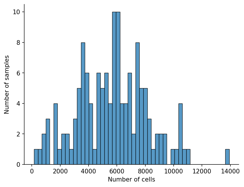
It is unlikely that a hundred cells is enough to obtain information about the sample, so we’ll filter out samples with too few cells. patpy provides a convenient function for that:

adata = patpy.pp.filter_small_samples(adata, sample_key=sample_key, sample_size_threshold=200)

1 samples removed: U00504-Ua005E-PBUa

If necessary, we can also remove cell types with too few cells in at least one sample:

adata = patpy.pp.filter_small_cell_groups(adata, sample_key=sample_key, cell_group_key=cell_type_key, cluster_size_threshold=10)

This typically leads to filtering out a lot of cell types, especially not very abundant ones. Some methods require this filtering step prior to building representation, but in this notebook we’ll focus on simpler methods that can be used with only sample filtering.

Simple sample representation baseline — Pseudobulk

Pseudobulk is the simplest sample representation: average every cell of a sample into a single vector. It can be interpreted as an “average cell” per sample. As simple as it is, pseudobulk is often a strong baseline. patpy provides a convenient interface to quickly run it.

But which cell representations should we use? In the literature, there is an inconsistency: some people prefer using gene expression, while other use latent features of the cells produced by dimensionality reduction methods. We can quickly test different cell representations by changing layer parameter

# Set up the sample representation method
pseudobulk_gene_expression = patpy.tl.Pseudobulk(
    sample_key=sample_key,
    cell_group_key=cell_type_key,  
    layer="X"  # Use adata.X that currently contains log-normalised expression
)
pseudobulk_gene_expression.prepare_anndata(adata)  # Prepare data
pseudobulk_gene_expression.calculate_distance_matrix(force=True);  # Compute sample representation

Per sample pseudobulks can now be accessed from the object:

pseudobulk_gene_expression.sample_representation

To pseudobulk a different layer, simply change the layer argument. patpy will take the data from a corresponding layer or .obsm slot. Additionally, .calculate_distance_matrix supports different aggregation functions (such as “sum” or “median”) and distance types, but changing them does not affect representations much.

pseudobulk_pca = patpy.tl.Pseudobulk(sample_key=sample_key, cell_group_key=cell_type_key, layer="X_pca")
pseudobulk_pca.prepare_anndata(adata)
pseudobulk_pca.calculate_distance_matrix(force=True);

Let’s try pseudobulking the latent space, and keep track of runtime to further compare it with other methods:

_t0 = _time.time()

pseudobulk_scvi = patpy.tl.Pseudobulk(sample_key=sample_key, cell_group_key=cell_type_key, layer="X_scVI_batch")
pseudobulk_scvi.prepare_anndata(adata)
pseudobulk_scvi.calculate_distance_matrix(force=True);

runtimes["combat"]["pseudobulk"] = _time.time() - _t0

It is convenient to store representations in an annotated data object (similarly to single-cell data). Take a look at anndata documentation if you are not familiar with it.

For sample-level analysis, it is handy to store pseudobulk gene expression in .X, metadata in .obs and sample representations in .obsm. Additionally, we’ll store sample representation names in a list in .uns to iterate over them later

meta_adata = pseudobulk_gene_expression.to_adata()
meta_adata.obs_names = pseudobulk_gene_expression.samples
meta_adata.var_names = adata.var_names # Set genes as var names
meta_adata.obs = metadata.loc[meta_adata.obs_names]
meta_adata

AnnData object with n_obs × n_vars = 137 × 3000
    obs: 'Source', 'Outcome', 'Death28', 'Institute', 'Pool_ID', 'Age', 'median_QC_ngenes', 'median_QC_pct_mitochondrial', 'median_QC_scrub_doublet_scores', 'n_cells', 'cell_type_B', 'cell_type_CD4', 'cell_type_CD8', 'cell_type_DC', 'cell_type_DN', 'cell_type_DP', 'cell_type_GDT', 'cell_type_HSC', 'cell_type_MAIT', 'cell_type_Mast', 'cell_type_NK', 'cell_type_PB', 'cell_type_PLT', 'cell_type_RET', 'cell_type_cMono', 'cell_type_iNKT', 'cell_type_ncMono'
    obsm: 'Pseudobulk'

Let’s define a small function to store all the necessary information in the correct slots and ensure that sample order is the same:

import numpy as np
import scanpy as sc

def store_representation(meta_adata, method, method_name):
    """
    Align sample representation with the rest of meta adata
    """
    
    representation_samples = list(method.samples)
    samples_order = [representation_samples.index(sample) for sample in meta_adata.obs_names if sample in representation_samples]
    assert (np.array(representation_samples)[samples_order] == meta_adata.obs_names).all(), "Order of samples is not correct"

    # meta_adata.obsm["umap"] = meta_adata.obsm[f"{method}_UMAP"]
    meta_adata.obsm[method_name] = np.array(method.sample_representation)[samples_order, :]
    meta_adata.obsm[f"{method_name}_distances"] = method.calculate_distance_matrix()[samples_order][:, samples_order]
    meta_adata.obsm[f"X_umap_{method_name}"] = method.embed("UMAP")[samples_order, :]

    # For technical reasons, we need to store distance matrix in obsm, and then run neighbors detection
    # It computes connectivities, and stores necessary slots in the right places
    sc.pp.neighbors(
        meta_adata, use_rep=f"{method_name}_distances", key_added=f"{method_name}_neighbors", metric="precomputed"
    )
    if "sample_representations" not in meta_adata.uns.keys():
        meta_adata.uns["sample_representations"] = []
        
    meta_adata.uns["sample_representations"].append(method_name)

    return meta_adata

meta_adata = store_representation(meta_adata, pseudobulk_gene_expression, "Pseudobulk_expression")

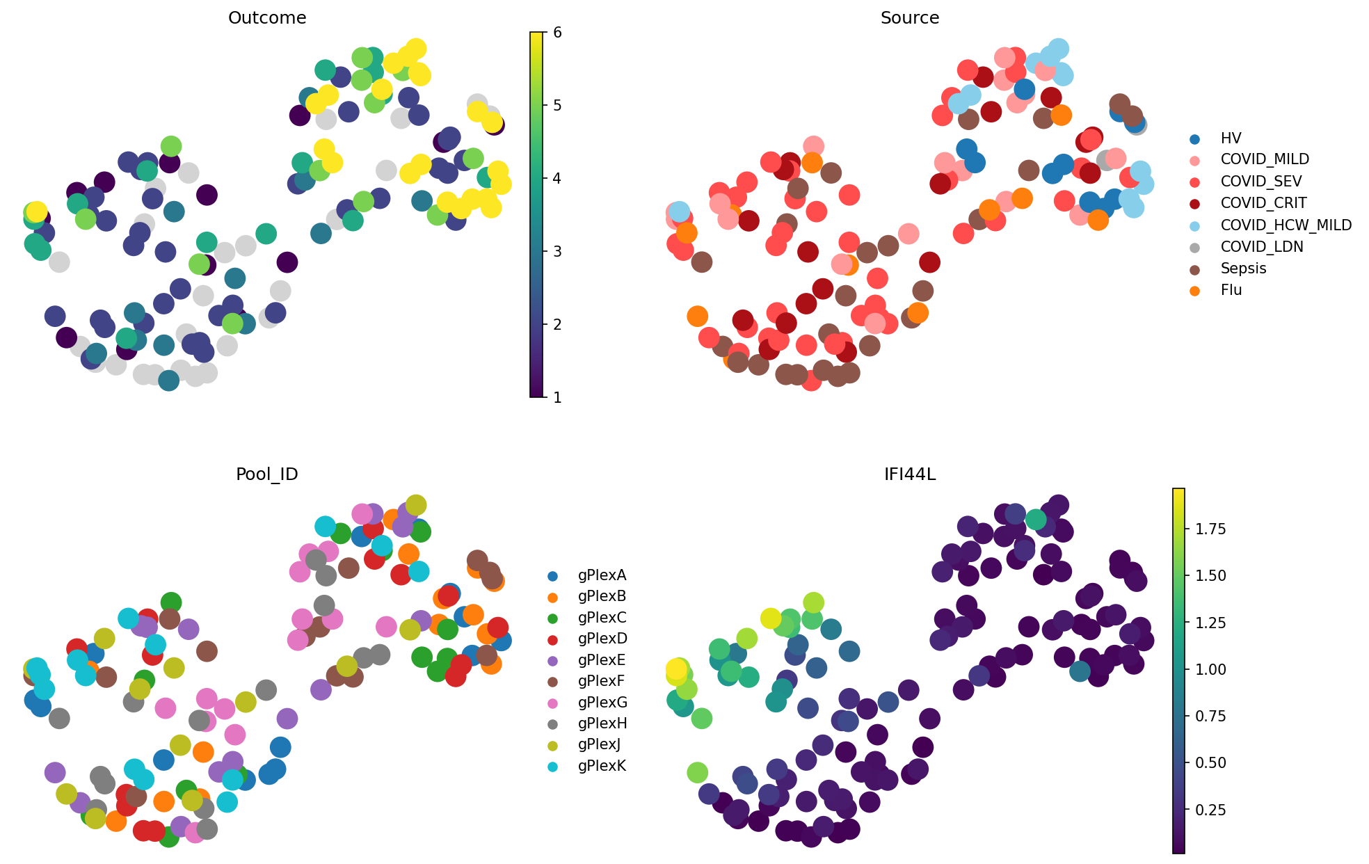
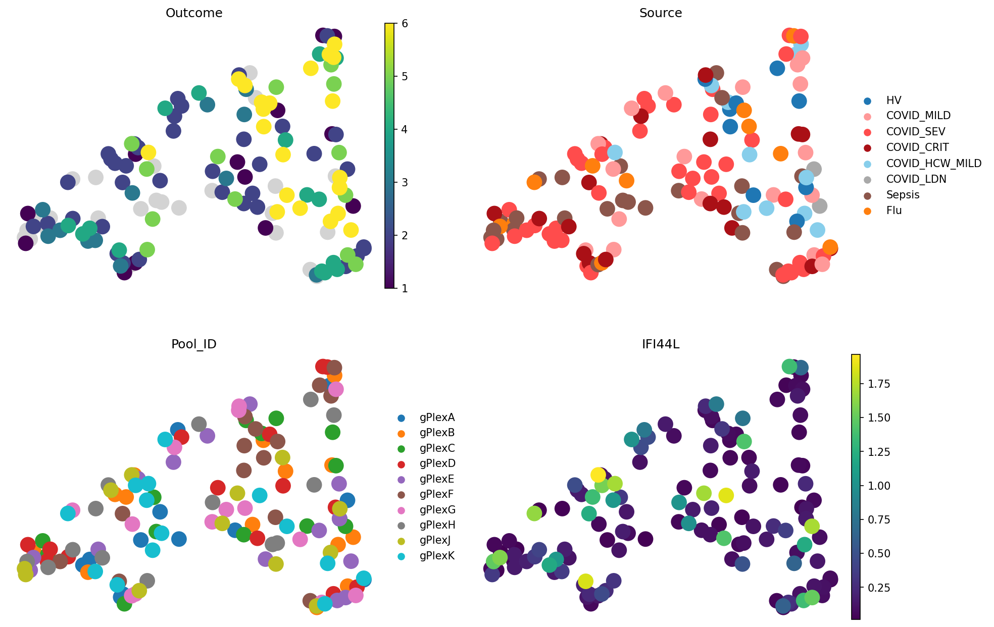
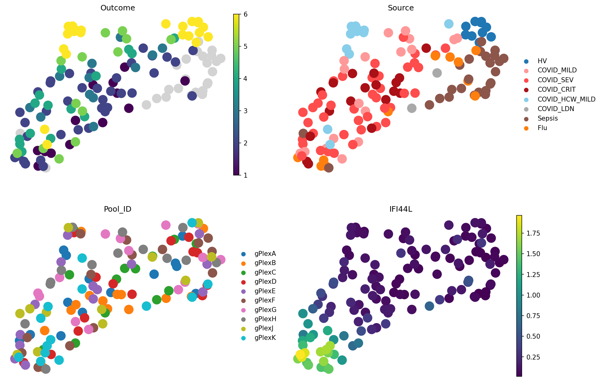
Representations can now easily be visualised using non-linear dimensionality reduction methods (such as UMAP). Note that every point on the plots below means one sample (i.e., patient ot a donor):

sc.pl.embedding(
    meta_adata,
    basis="X_umap_Pseudobulk_expression", 
    color=["Outcome", "Source", "Pool_ID", "IFI44L"],  # Both metadata columns and gene expression can be visualised. IFI44L is a COVID-19 marker
    frameon=False,
    ncols=2
)

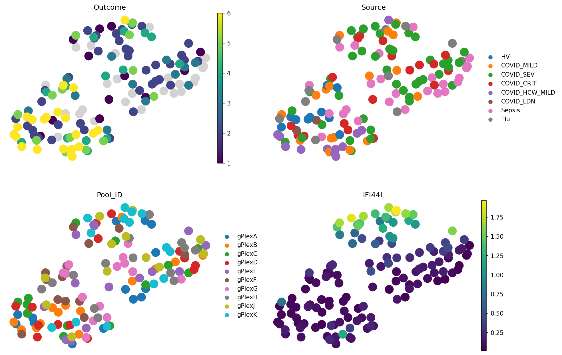
The “Outcome” plot in the top left reflects different severities of COVID-19. It decodes the following:

1 = Death
2 = Intubated, ventilated
3 = Non-invasive ventilation
4 = Hospitalized, O2
5 = Hospitalized, no O2
6 = Not hospitalized

We can see that people with outcome 6 are mostly close to each other, which is a good sign. Source plot shows a similar story, but additionally shows Flu and Sepsis samples. Pool ID doesn’t show grouping, which is good news because this is a batch covariate.

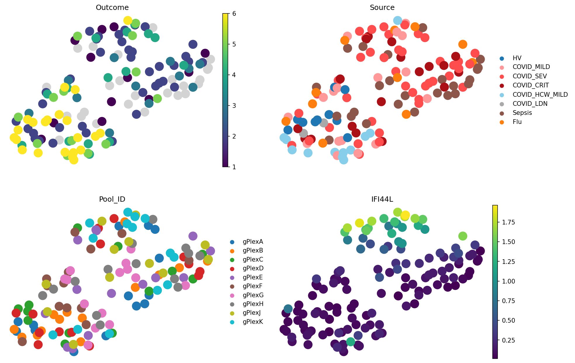
We can define more intuitive palettes and store them in .uns for consistent coloring across methods:

meta_adata.obs["Source"].cat.categories

Index(['HV', 'COVID_MILD', 'COVID_SEV', 'COVID_CRIT', 'COVID_HCW_MILD',
       'COVID_LDN', 'Sepsis', 'Flu'],
      dtype='object')

meta_adata.uns["Source_colors"] = [
    "#1f77b4",  # HV
    "#ff9999",  # COVID_MILD
    "#ff4c4c",  # COVID_SEV
    sns.color_palette("Reds")[-1],  # COVID_CRIT
    "skyblue", # COVID_HCW_MILD
    "darkgrey", # COVID_LDN
    "#8c564b",  # Sepsis
    "#ff7f0e",  # Flu
]

sc.pl.embedding(
    meta_adata,
    basis="X_umap_Pseudobulk_expression", 
    color=["Outcome", "Source", "Pool_ID", "IFI44L"],
    frameon=False,
    ncols=2
)

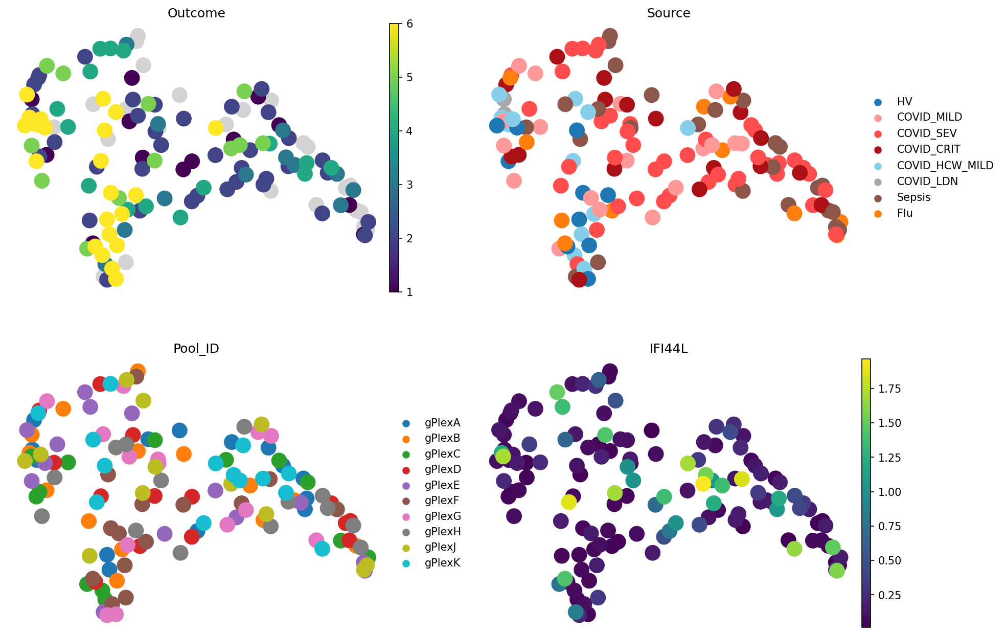
Let’s see what PCA-based representation shows us:

meta_adata = store_representation(meta_adata, pseudobulk_pca, "Pseudobulk_PCA")

sc.pl.embedding(
    meta_adata,
    basis="X_umap_Pseudobulk_PCA", 
    color=["Outcome", "Source", "Pool_ID", "IFI44L"],
    frameon=False,
    ncols=2
)

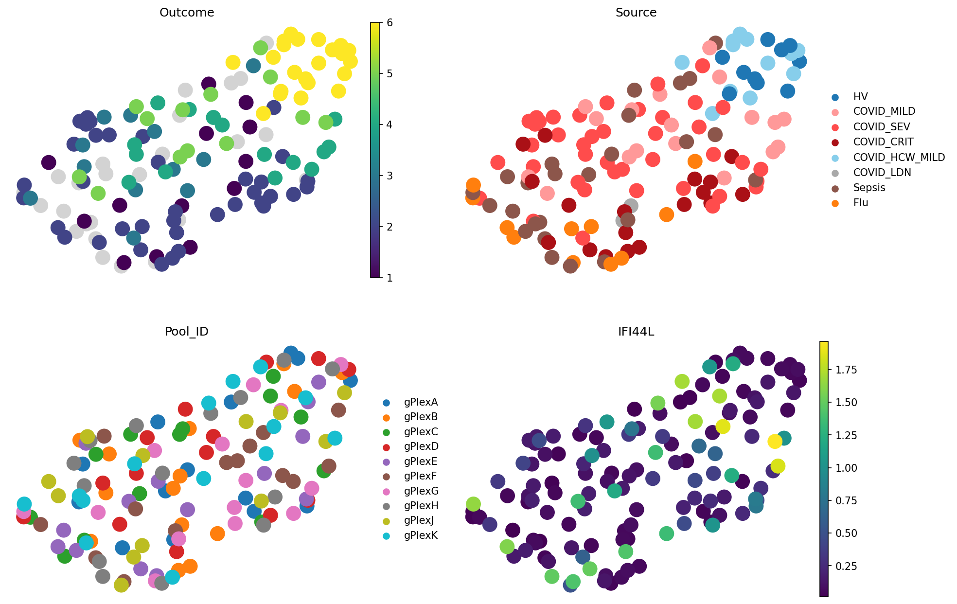
PCA-based representations tell a similar story. What about scVI?

meta_adata = store_representation(meta_adata, pseudobulk_scvi, "Pseudobulk_scVI")

sc.pl.embedding(
    meta_adata,
    basis="X_umap_Pseudobulk_scVI", 
    color=["Outcome", "Source", "Pool_ID", "IFI44L"],
    frameon=False,
    ncols=2
)

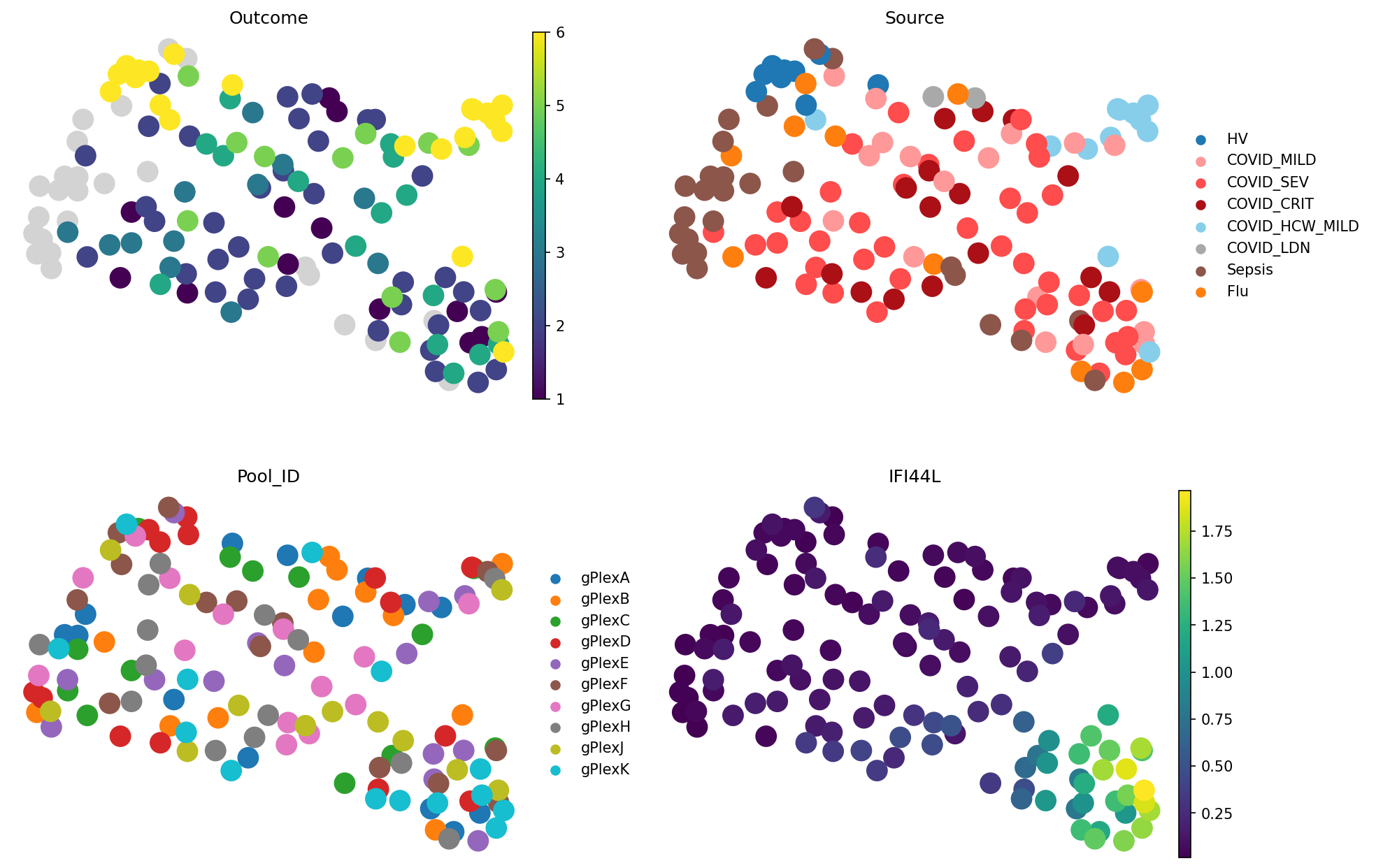
Here, we can notice a better grouping of Sources (e.g. Sepsis, and healthy) as well as the outcomes. Interestingly, outcome 6 (not hospitalised) now splits into 2 groups. On the Source plot, we can see that they correspond to different groups: HV (healthy volunteers) and “COVID_HCW_MILD”, which encodes healthcare workers dealing with COVID-19 patients. The Pool ID plot shows that these samples come from diverse batches, so the difference is likely biological rather than technical. Immune system of healthcare workers exposed to COVID-19 contains slightly different signture, which is consistently captured by pseudobulking in scVI space, but not in PCA or gene expression.

Long story short, data preprocessing matters for sample representations. With good cell embeddigns, such as scVI, even the simplest methods can uncover patient diversity.

But let’s stop staring on the UMAPs and compute some metrics. 2D visualisations of complex data give you some hint on what it’s hiding, but should never be overinterpreted.

Evaluating biological information retention and batch mixing in sample representations

What do we expect from a good sample representation? Briefly, we want biologically similar samples to be close to each other in sample representation space. At the same time, we don’t want similarity to be explained by batch effects. We previously proposed evaluating both points with k nearest neighbors (KNN)-based prediction:

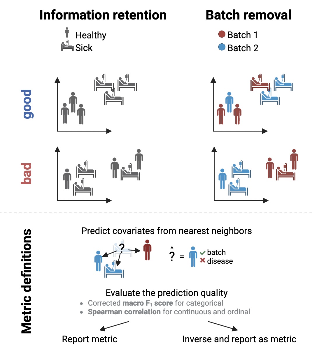
Approach is simple: predict each covariate from the most similar samples. Evaluate how well it corresponds to true values. For biological covariates, report the prediction quality. For technical, inverse it so that 1 corresponds to perfect mixing, and 0 corresponds to perfect batch prediction.

patpy provides a simple interface to these metrics. Let’s see how well we can predict the outcome from pseudobulk representations:

pseudobulk_gene_expression.evaluate_representation(target="Outcome", method="knn", n_neighbors=5, task="classification")

{'score': np.float64(0.1958570399511462),
 'metric': 'f1_macro_calibrated',
 'n_unique': 6,
 'n_observations': 112,
 'method': 'knn'}

Here, we can see that based on 5 most similar samples, Outcome cannot be predicted so well. For the classification task, $F_1$-macro score is used. This metrics weighs each class equally. It is also calibrated for random prediction so that 0 means that the prediction score is as good as throwing random classes, and 1 means perfect prediction.

Outcome in our data is, however, encoded numerically. We might want to use this information. For example, if the most similar samples have outcome values [6, 6, 6, 4, 4], predicting 5 is much better than predicting 1. Let’s change the prediction task from classification (requiring the exact prediction of the class) to ranking, which takes into accout how far the prediction was from the correct class:

pseudobulk_gene_expression.evaluate_representation(target="Outcome", method="knn", n_neighbors=5, task="ranking")

{'score': np.float64(0.5822470283432646),
 'metric': 'spearman_r',
 'n_unique': 6,
 'n_observations': 112,
 'method': 'knn'}

We can see that prediction is not that terrible. Note that the metric changed to Spearman correlation. Interpretation is the same: 0 means poor prediction while 1 would correspond to a perfect ranking of outcomes.

Now let’s see how well samples Pool is represented. This is a technical covariate so we don’t want score to be high:

pseudobulk_gene_expression.evaluate_representation(target="Pool_ID", method="knn", n_neighbors=5, task="classification")

{'score': np.float64(0.24192529778333363),
 'metric': 'f1_macro_calibrated',
 'n_unique': 10,
 'n_observations': 137,
 'method': 'knn'}

The value is quite low, so the batch effect does not strongly affect this representation.

We can also test whether continuous covatiates, such as the number of cells drive the representation. For this, use the regression task. Note that the number of cells is not stored in adata (where other covariates are taken from), so we need to explicitly provide the metadata table:

pseudobulk_gene_expression.evaluate_representation(
    metadata=metadata.loc[pseudobulk_gene_expression.samples],
    target="n_cells", 
    method="knn", 
    n_neighbors=5, 
    task="regression"
)

{'score': np.float64(0.2638191423824369),
 'metric': 'spearman_r',
 'n_unique': 137,
 'n_observations': 137,
 'method': 'knn'}

Good news, the number of cells affects the sample representations much less than the outcome!

We can now see which input space better captures biology and is more resistant to batch effects:

scores = []

for method, input_space in zip([pseudobulk_gene_expression, pseudobulk_pca, pseudobulk_scvi], ["expression", "PCA", "scVI"]):
    outcome_score = method.evaluate_representation(target="Outcome", method="knn", n_neighbors=5, task="ranking")["score"]
    n_cells_score = method.evaluate_representation(metadata=metadata.loc[pseudobulk_gene_expression.samples], target="n_cells", method="knn", n_neighbors=5, task="regression")["score"]
    # Inverse technical score
    n_cells_score = 1 - n_cells_score
    scores.append([input_space, outcome_score, n_cells_score])

input_space_results = pd.DataFrame(scores, columns=["Input space", "Outcome prediction", "#cells mixing"])
input_space_results

	Input space	Outcome prediction	#cells mixing
0	expression	0.582247	0.736181
1	PCA	0.575498	0.725148
2	scVI	0.612422	0.647115

sns.scatterplot(input_space_results, x="Outcome prediction", y="#cells mixing", hue="Input space", s=200)

<Axes: xlabel='Outcome prediction', ylabel='#cells mixing'>

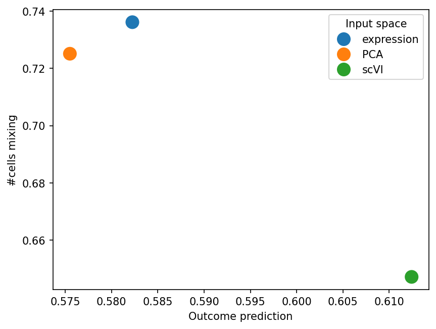
The results are not drastically different, but scVI captures Outcome slightly better. Note, however, that it is also affected by the number of cells.

Silhouette score, another commonly used metric, is also supported by patpy. However, it does not enable evaluating continuous or ranked covariates. Let’s still see if it shows us the similar picture:

method.evaluate_representation(target="Pool_ID", method="silhouette")

{'score': -0.049224236460995476,
 'metric': 'silhouette',
 'n_unique': 10,
 'n_observations': 137,
 'method': 'silhouette'}

silhouette_scores = []

for method, input_space in zip([pseudobulk_gene_expression, pseudobulk_pca, pseudobulk_scvi], ["expression", "PCA", "scVI"]):
    outcome_score = method.evaluate_representation(target="Outcome", method="silhouette")["score"]
    pool_id_score = method.evaluate_representation(target="Pool_ID", method="silhouette")["score"]
    silhouette_scores.append([input_space, outcome_score, pool_id_score])

input_space_silhouette_results = pd.DataFrame(silhouette_scores, columns=["Input space", "Outcome clustering", "Pool clustering"])
input_space_silhouette_results

	Input space	Outcome clustering	Pool clustering
0	expression	-0.078705	-0.056767
1	PCA	-0.085367	-0.070996
2	scVI	-0.057449	-0.049224

sns.scatterplot(input_space_silhouette_results, x="Outcome clustering", y="Pool clustering", hue="Input space", s=200)

<Axes: xlabel='Outcome clustering', ylabel='Pool clustering'>

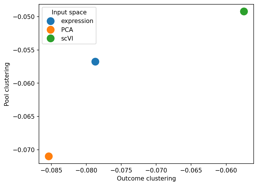
Near 0 (and even slightly negative) silhouette metric values show us that both outcome and pools are not separated in the sample representation. This is expected from what we saw on UMAPs: groups mix a lot rather that showing completely separate clusters. It does not, however, mean that pseudobulk representations do not reflect biology. As we saw from kNN-based metrics, the representations are locally meningful and enable prediction of clinical covariates, such as the outcome.

Let’s use another metric to see if COVID-19 severity is preserved in sample representations.

Evaluating trajectory preservation in sample representations

Besides local predictability of sample representations, we also want sample embeddings to have a meaningful global structure. When there is a ground truth trajectory in our data, such as disease severity, we can evaluate if samples are ordered correspondingly to this trajectory:

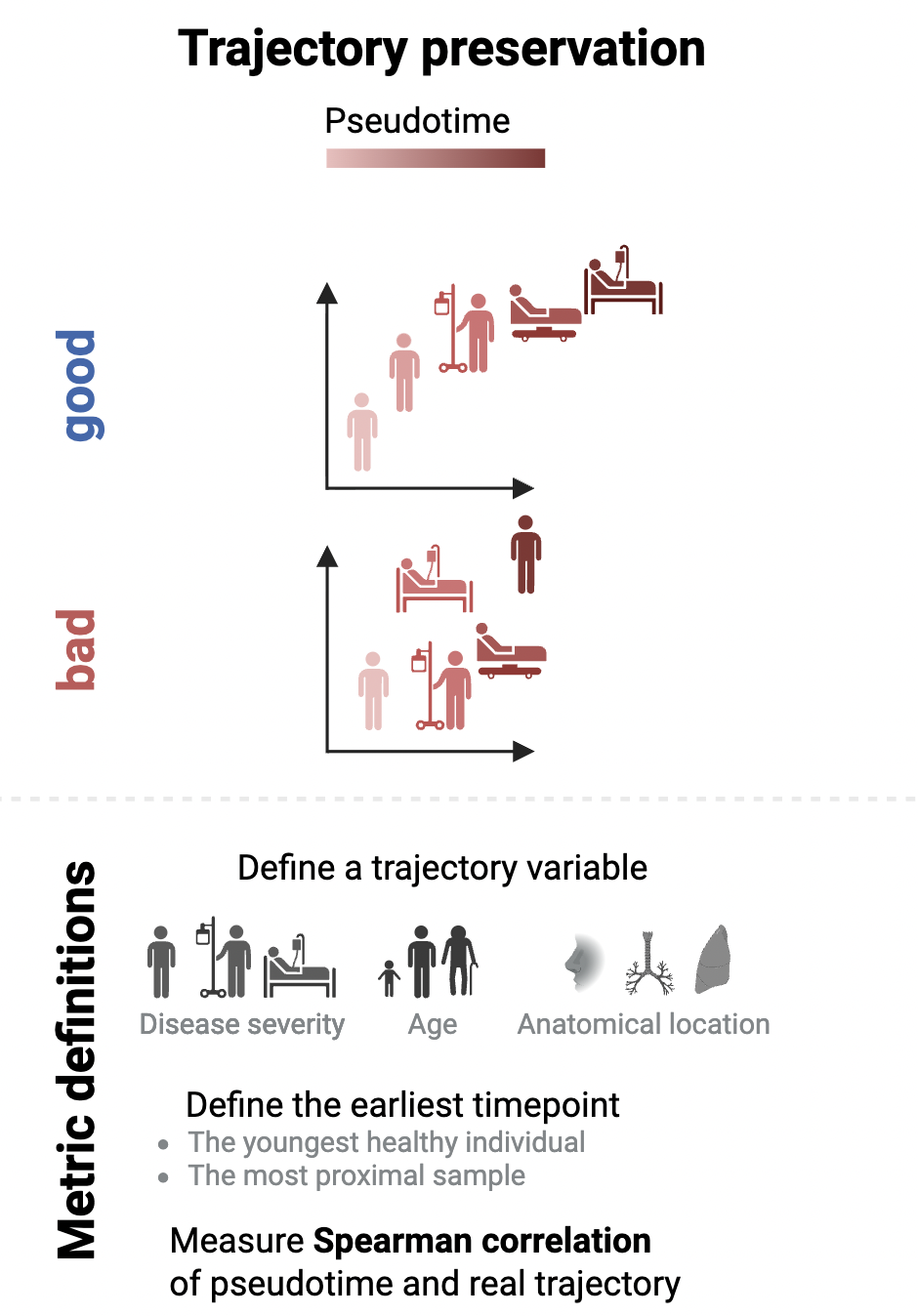
First, we need to set a “root sample” – the beginning of our trajectory. The youngest control donor is a reasonable choice:

adata.obs["Age"]

AAACCTGAGAAAGTGG-1-gPlexA1    5.0
AAACCTGAGCGGATCA-1-gPlexA1    5.0
AAACCTGAGGCGACAT-1-gPlexA1    7.0
AAACCTGAGGGAACGG-1-gPlexA1    5.0
AAACCTGCACATGTGT-1-gPlexA1    7.0
                             ... 
TTTGTCAGTGGCAAAC-1-gPlexK7    6.0
TTTGTCAGTTACCGAT-1-gPlexK7    6.0
TTTGTCATCCTCTAGC-1-gPlexK7    4.0
TTTGTCATCGAGGTAG-1-gPlexK7    7.0
TTTGTCATCTCCCTGA-1-gPlexK7    7.0
Name: Age, Length: 783516, dtype: float64

candidates = metadata.dropna(subset=["Outcome", "Age"])
root_sample = candidates.sort_values(["Outcome", "Age"], ascending=[False, True]).index[0]
print(
    f"Trajectory root: {root_sample} "
    f"(Outcome={metadata.loc[root_sample, 'Outcome']:.0f}, "
    f"Age={metadata.loc[root_sample, 'Age']:.0f}, "
    f"Source={metadata.loc[root_sample, 'Source']})"
)

Trajectory root: G05078-Ja005E-PBCa (Outcome=6, Age=3, Source=COVID_HCW_MILD)

trajectory_results = patpy.tl.trajectory_correlation(
    meta_adata=meta_adata,
    root_sample=root_sample,
    trajectory_variable="Outcome",
    representations=meta_adata.uns["sample_representations"],
    inverse_trajectory=True,  # COMBAT codes 6 = healthy, 1 = critical, so we need to flip the sign for correlation with pseudotime
)
trajectory_results

Computing diffmap for Pseudobulk_expression
Computing diffmap for Pseudobulk_PCA
Computing diffmap for Pseudobulk_scVI

	correlation
Pseudobulk_expression	0.459593
Pseudobulk_PCA	0.450696
Pseudobulk_scVI	0.400080

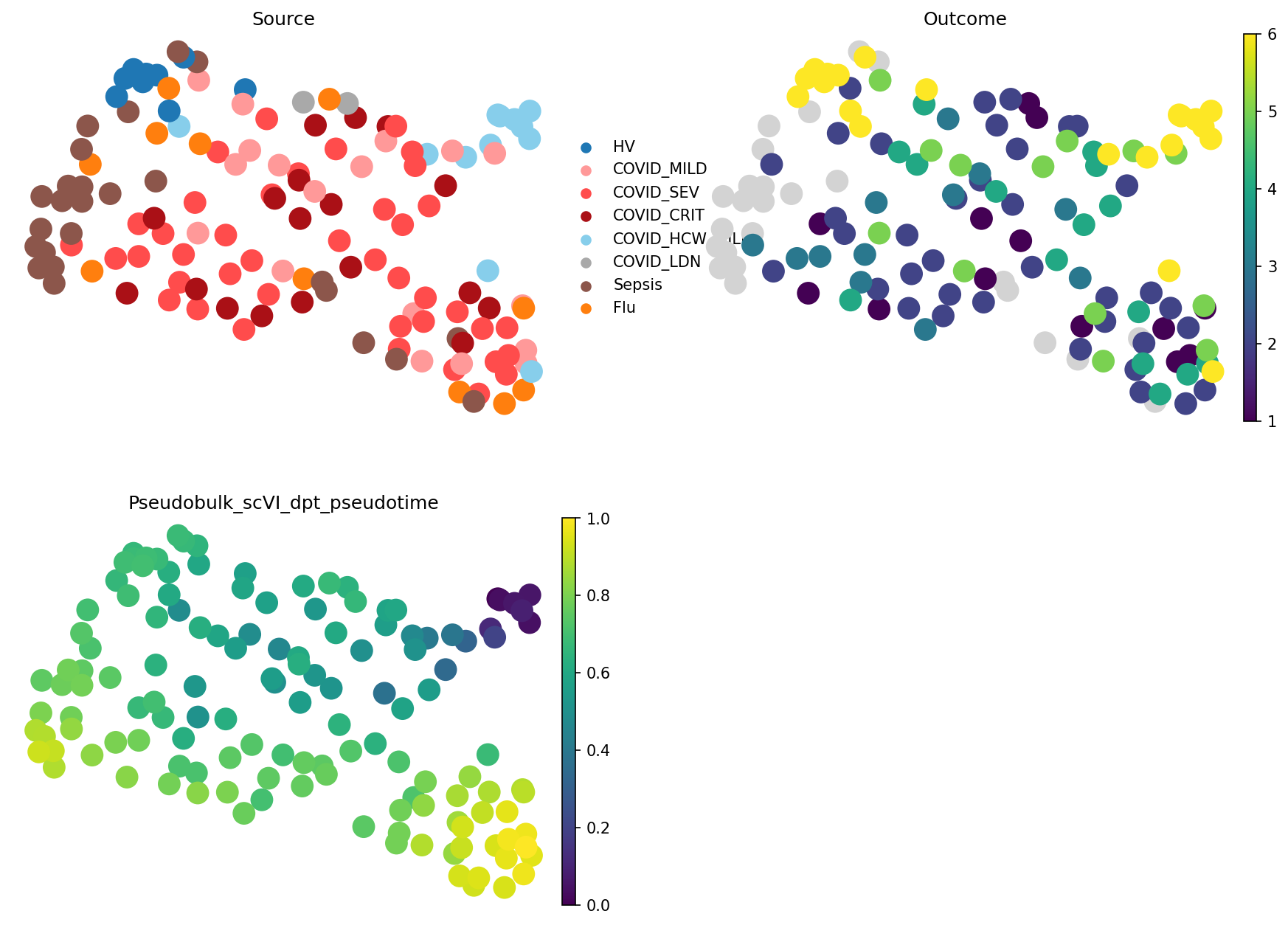
We can see that expression-based pseudobulk captures trajectory even better. This is likely due to split between healthcare workers and healthy volunteers in scVI-based representation. We can visualise pseudotime to see it:

sc.pl.embedding(
    meta_adata,
    basis="X_umap_Pseudobulk_scVI", 
    color=["Source", "Outcome", "Pseudobulk_scVI_dpt_pseudotime"],
    frameon=False,
    ncols=2
)

sc.pl.embedding(
    meta_adata,
    basis="X_umap_Pseudobulk_expression", 
    color=["Source", "Outcome", "Pseudobulk_expression_dpt_pseudotime"],
    frameon=False,
    ncols=2
)

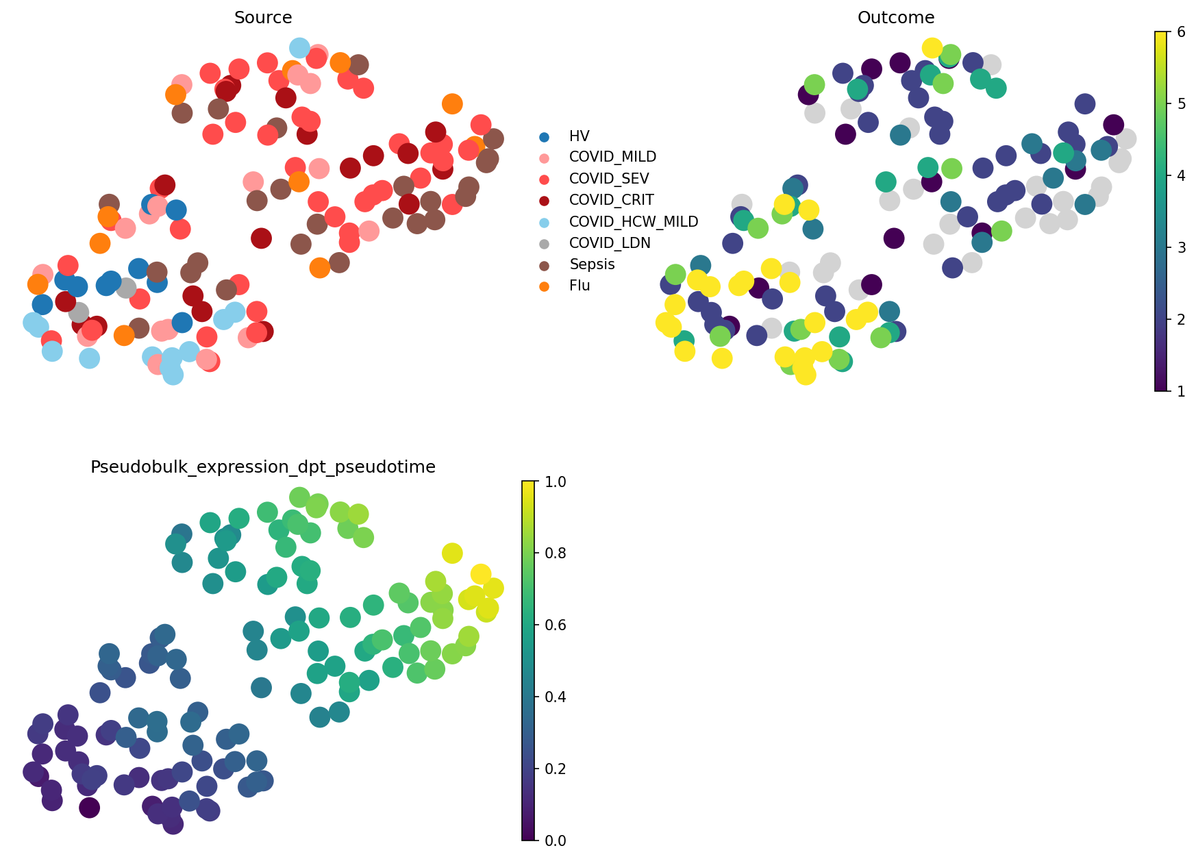
Indeed, we see that in scVI-based embedding, pseudotime took a wrong turn to the healthy cluster, while expression-based pseudobulk groups all samples with the good outcome together. What’s right and what’s wrong depends on your research question. For modelling patient trajectories, expression-based embedding would be better, while for understanding COVID-19 response diversity, scVI shows a better picture

Method 2 — Cell type composition

Another commonly used baseline representation is based on cell type composition differences. It is calculated as a difference between cell type proportions in each sample.

_t0 = _time.time()
composition = patpy.tl.CellGroupComposition(
    sample_key=sample_key, cell_group_key=cell_type_key,
)
composition.prepare_anndata(adata)
composition_distances = composition.calculate_distance_matrix(force=True)
runtimes["combat"]["composition"] = _time.time() - _t0

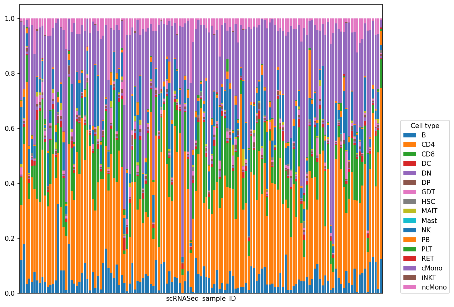
We can also visualise cell type proportions for each sample:

composition.sample_representation.plot(kind="bar", stacked=True, figsize=(10, 8), width=0.8)
plt.xticks([])
plt.legend(loc=(1.05, 0), title="Cell type");

meta_adata = store_representation(meta_adata, composition, "composition")

sc.pl.embedding(
    meta_adata,
    basis="X_umap_composition", 
    color=["Outcome", "Source", "Pool_ID", "IFI44L"],
    frameon=False,
    ncols=2
)

We can see that cell type composition reflects patient outcome worse than pseudobulk:

composition.evaluate_representation(target="Outcome", method="knn", n_neighbors=5, task="ranking")

{'score': np.float64(0.4786968063752981),
 'metric': 'spearman_r',
 'n_unique': 6,
 'n_observations': 112,
 'method': 'knn'}

However, a better way to compare samples based on compositional data is by applying centered log-ratio (CLR) transformation to the cell type composition. This approach is know in the sample representation literature as SETA or scECODA. patpy enables CLR transform with a single extra argument:

_t0 = _time.time()
composition_clr = patpy.tl.CellGroupComposition(
    sample_key=sample_key, cell_group_key=cell_type_key, 
    apply_clr=True # Transform proportions with centered log-ratio
)
composition_clr.prepare_anndata(adata)
composition_clr.calculate_distance_matrix(force=True)
runtimes["combat"]["composition_clr"] = _time.time() - _t0

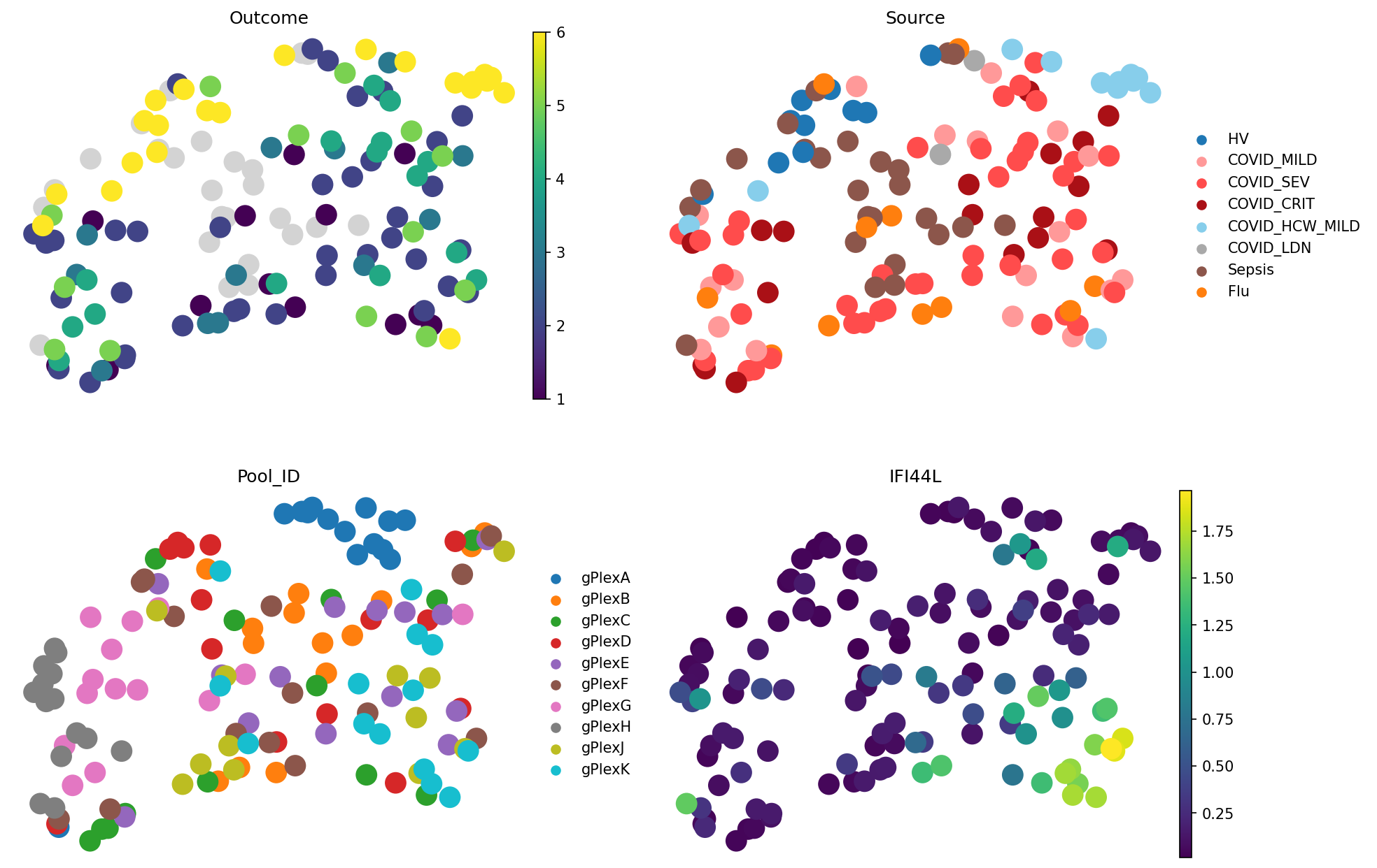
meta_adata = store_representation(meta_adata, composition_clr, "composition_clr")

sc.pl.embedding(
    meta_adata,
    basis="X_umap_composition_clr", 
    color=["Outcome", "Source", "Pool_ID", "IFI44L"],
    frameon=False,
    ncols=2
)

CLR-transformed cell type proportions give us the best representation we saw so far! Although, note how IFI44L gene expression gets distributed across the embedding. It makes sense as this method does not distinguish samples with same cell type proportions but different gene expression

composition_clr.evaluate_representation(target="Outcome", method="knn", n_neighbors=5, task="ranking")

{'score': np.float64(0.6751412180597196),
 'metric': 'spearman_r',
 'n_unique': 6,
 'n_observations': 112,
 'method': 'knn'}

Method 3 — PILOT

PILOT is an Optimal Transport-based tool, which calculates distances between samples based on cell type proportion differences taking into account cell type similarities. Note that to run it, you need to install the dependencies additionally:

pip install patpy[pilot]

_t0 = _time.time()
pilot = patpy.tl.PILOT(
    sample_key=sample_key,
    cell_group_key=cell_type_key,
    layer="X_scVI_batch",
    sample_state_col="Outcome",  # not used for distance calculation
)
pilot.prepare_anndata(adata)
pilot.calculate_distance_matrix()
runtimes["combat"]["pilot"] = _time.time() - _t0
meta_adata = store_representation(meta_adata, pilot, "pilot")

sc.pl.embedding(
    meta_adata,
    basis="X_umap_pilot", 
    color=["Outcome", "Source", "Pool_ID", "IFI44L"],
    frameon=False,
    ncols=2
)

We can see that for COMBAT dataset and outcome signal preservation, PILOT does not outperform simpler baselines:

pilot.evaluate_representation(target="Outcome", method="knn", n_neighbors=5, task="ranking")

{'score': np.float64(0.49516263715930153),
 'metric': 'spearman_r',
 'n_unique': 6,
 'n_observations': 112,
 'method': 'knn'}

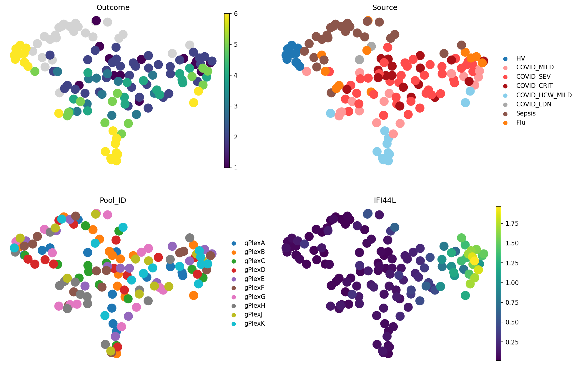
Method 4 — GroupedPseudobulk

GroupedPseudobulk is one step richer than Pseudobulk: instead of one vector per sample, you get one vector per cell type per sample, then concatenate them. If your biological signal in some cell types respond differently than the global average, this representation will uncover it. Moreover, grouped pseudobulk does not take into account cell type proportion differences, which can be beneficial, when cell type composition is explained by noise rather than by biology

Unlike plain Pseudobulk, this method needs at least a few cells in every (sample, cell_type) pair, so we drop very sparse cell types via patpy.pp.filter_small_cell_groups:

adata_for_grouped = patpy.pp.filter_small_cell_groups(
    adata,
    sample_key=sample_key,
    cell_group_key=cell_type_key,
    cluster_size_threshold=5,
)

13 cell types removed: DP, PB, HSC, ncMono, DC, GDT, DN, RET, MAIT, B, iNKT, Mast, PLT

_t0 = _time.time()

grouped_pseudobulk = patpy.tl.GroupedPseudobulk(
    sample_key=sample_key,
    cell_group_key=cell_type_key,
    layer="X_scVI_batch",
)
grouped_pseudobulk.prepare_anndata(adata_for_grouped)
grouped_pseudobulk.calculate_distance_matrix();

runtimes["combat"]["grouped_pseudobulk"] = _time.time() - _t0

# So far, sample_representation contains pseudobulks for each of cell types
# Let's concatenate them for each sample to have 1 vector per sample
grouped_pseudobulk.sample_representation = np.concatenate(grouped_pseudobulk.sample_representation, axis=0)

meta_adata = store_representation(meta_adata, grouped_pseudobulk, "grouped_pseudobulk")

sc.pl.embedding(
    meta_adata,
    basis="X_umap_grouped_pseudobulk", 
    color=["Outcome", "Source", "Pool_ID", "IFI44L"],
    frameon=False,
    ncols=2
)

Despite losing a lot of information about sparse cell types and cell type composition, this is the best representation we saw so far:

grouped_pseudobulk.evaluate_representation(target="Outcome", method="knn", n_neighbors=5, task="ranking")

{'score': np.float64(0.7346012837763595),
 'metric': 'spearman_r',
 'n_unique': 6,
 'n_observations': 112,
 'method': 'knn'}

Method 5 — RandomVector (sanity baseline)

RandomVector assigns each sample a vector of Gaussian noise. It exists as a floor for the comparison table: any real method should beat random on the clinical covariates and should not beat random on the technical ones. It is also a good sanity check for overinterpretation of UMAPs. If you show some people sample representation of this method and they start to see patterns, do not show them UMAPs anymore

_t0 = _time.time()
random_vec = patpy.tl.RandomVector(
    sample_key=sample_key,
    cell_group_key=cell_type_key,
)
random_vec.prepare_anndata(adata)
random_vec.calculate_distance_matrix();
runtimes["combat"]["random_vec"] = _time.time() - _t0

meta_adata = store_representation(meta_adata, random_vec, "random_vec")

sc.pl.embedding(
    meta_adata,
    basis="X_umap_random_vec", 
    color=["Outcome", "Source", "Pool_ID", "IFI44L"],
    frameon=False,
    ncols=2
)

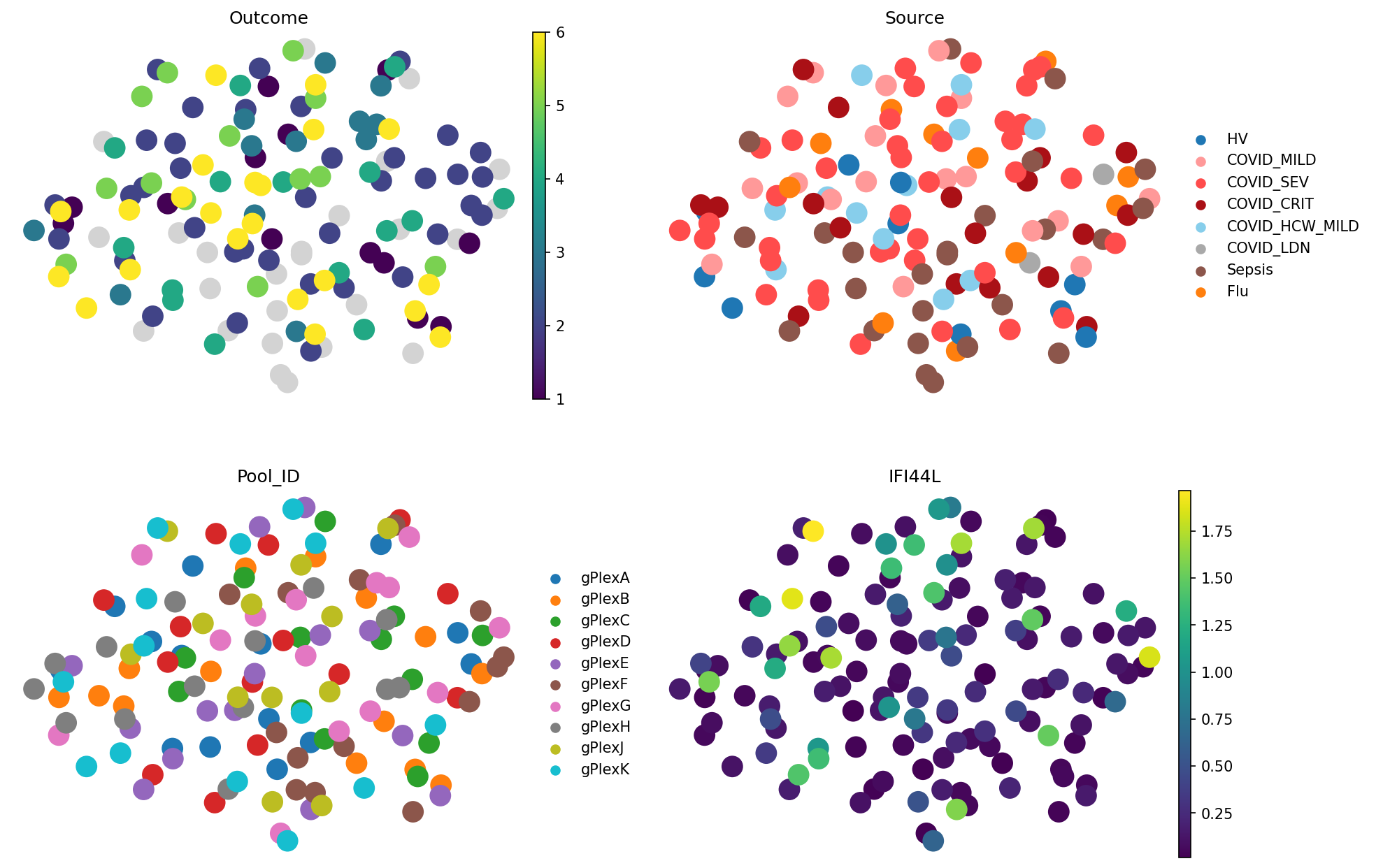
Do you see this group on the right? No? That’s right, there is no structure here beyond noise. Metrics show it clearly:

random_vec.evaluate_representation(target="Outcome", method="knn", n_neighbors=5, task="ranking")

{'score': np.float64(0.0),
 'metric': 'spearman_r',
 'n_unique': 6,
 'n_observations': 112,
 'method': 'knn'}

Method 6 — MOFA

MOFA2 fits a multi-view factor model: each cell type becomes a view, and shared latent factors are inferred across views

Requires pip install mofapy2 (no [mofa] extra in patpy yet).

_t0 = _time.time()
mofa = patpy.tl.MOFA(
    sample_key=sample_key,
    cell_group_key=cell_type_key,
    n_factors=10,
    aggregate_cell_types=True,
    layer="X"
)
mofa.prepare_anndata(adata_for_grouped) # MOFA aggregates cells per cell type and samples too, so provide filtered adata
mofa.calculate_distance_matrix();
runtimes["combat"]["mofa"] = _time.time() - _t0

        #########################################################
        ###           __  __  ____  ______                    ### 
        ###          |  \/  |/ __ \|  ____/\    _             ### 
        ###          | \  / | |  | | |__ /  \ _| |_           ### 
        ###          | |\/| | |  | |  __/ /\ \_   _|          ###
        ###          | |  | | |__| | | / ____ \|_|            ###
        ###          |_|  |_|\____/|_|/_/    \_\              ###
        ###                                                   ### 
        #########################################################
Features names not provided, using default naming convention:
- feature1_view1, featureD_viewM

Successfully loaded view='NK' group='group1' with N=137 samples and D=3000 features...
Successfully loaded view='CD8' group='group1' with N=137 samples and D=3000 features...
Successfully loaded view='cMono' group='group1' with N=137 samples and D=3000 features...
Successfully loaded view='CD4' group='group1' with N=137 samples and D=3000 features...


Warning: 341 features(s) in view 0 have zero variance, consider removing them before training the model...
Warning: 237 features(s) in view 1 have zero variance, consider removing them before training the model...
Warning: 130 features(s) in view 2 have zero variance, consider removing them before training the model...
Warning: 102 features(s) in view 3 have zero variance, consider removing them before training the model...
Model options:
- Automatic Relevance Determination prior on the factors: False
- Automatic Relevance Determination prior on the weights: True
- Spike-and-slab prior on the factors: False
- Spike-and-slab prior on the weights: True
Likelihoods:
- View 0 (NK): gaussian
- View 1 (CD8): gaussian
- View 2 (cMono): gaussian
- View 3 (CD4): gaussian


######################################
## Training the model with seed 67 ##
######################################


ELBO before training: -12030533.85
Iteration 1: time=0.14, ELBO=2796110.12, deltaELBO=14826643.964 (123.24177924%), Factors=10
Iteration 2: time=0.11, ELBO=4886898.14, deltaELBO=2090788.025 (17.37901286%), Factors=10
Iteration 3: time=0.11, ELBO=4966654.48, deltaELBO=79756.333 (0.66294924%), Factors=10
Iteration 4: time=0.11, ELBO=5016306.24, deltaELBO=49651.762 (0.41271454%), Factors=10
Iteration 5: time=0.11, ELBO=5034083.69, deltaELBO=17777.458 (0.14776948%), Factors=10
Iteration 6: time=0.11, ELBO=5052142.81, deltaELBO=18059.111 (0.15011064%), Factors=10
Iteration 7: time=0.11, ELBO=5064988.89, deltaELBO=12846.083 (0.10677900%), Factors=10
Iteration 8: time=0.11, ELBO=5071148.78, deltaELBO=6159.892 (0.05120215%), Factors=10
Iteration 9: time=0.10, ELBO=5075410.43, deltaELBO=4261.652 (0.03542363%), Factors=10
Iteration 10: time=1.48, ELBO=5079015.25, deltaELBO=3604.812 (0.02996386%), Factors=10
Iteration 11: time=0.09, ELBO=5082066.07, deltaELBO=3050.822 (0.02535899%), Factors=10
Iteration 12: time=0.09, ELBO=5084730.69, deltaELBO=2664.625 (0.02214885%), Factors=10
Iteration 13: time=0.09, ELBO=5086855.70, deltaELBO=2125.005 (0.01766343%), Factors=10
Iteration 14: time=0.09, ELBO=5088622.75, deltaELBO=1767.051 (0.01468805%), Factors=10
Iteration 15: time=0.09, ELBO=5090236.52, deltaELBO=1613.772 (0.01341396%), Factors=10
Iteration 16: time=0.09, ELBO=5091771.17, deltaELBO=1534.654 (0.01275633%), Factors=10
Iteration 17: time=0.09, ELBO=5093268.27, deltaELBO=1497.095 (0.01244413%), Factors=10
Iteration 18: time=0.09, ELBO=5094740.59, deltaELBO=1472.325 (0.01223824%), Factors=10
Iteration 19: time=0.09, ELBO=5096200.20, deltaELBO=1459.601 (0.01213247%), Factors=10
Iteration 20: time=0.09, ELBO=5097640.91, deltaELBO=1440.719 (0.01197552%), Factors=10
Iteration 21: time=0.09, ELBO=5099012.97, deltaELBO=1372.054 (0.01140476%), Factors=10
Iteration 22: time=0.09, ELBO=5100265.04, deltaELBO=1252.071 (0.01040744%), Factors=10
Iteration 23: time=0.09, ELBO=5101413.24, deltaELBO=1148.203 (0.00954407%), Factors=10
Iteration 24: time=0.09, ELBO=5102487.84, deltaELBO=1074.603 (0.00893230%), Factors=10
Iteration 25: time=0.09, ELBO=5103499.83, deltaELBO=1011.983 (0.00841179%), Factors=10
Iteration 26: time=0.09, ELBO=5104446.48, deltaELBO=946.653 (0.00786876%), Factors=10
Iteration 27: time=0.09, ELBO=5105326.49, deltaELBO=880.009 (0.00731479%), Factors=10
Iteration 28: time=0.09, ELBO=5106151.71, deltaELBO=825.215 (0.00685934%), Factors=10
Iteration 29: time=0.09, ELBO=5106942.58, deltaELBO=790.874 (0.00657389%), Factors=10
Iteration 30: time=0.09, ELBO=5107699.48, deltaELBO=756.900 (0.00629149%), Factors=10
Iteration 31: time=0.08, ELBO=5108424.16, deltaELBO=724.676 (0.00602364%), Factors=10
Iteration 32: time=0.08, ELBO=5109119.26, deltaELBO=695.106 (0.00577785%), Factors=10
Iteration 33: time=0.07, ELBO=5109782.30, deltaELBO=663.037 (0.00551129%), Factors=10
Iteration 34: time=0.07, ELBO=5110416.62, deltaELBO=634.317 (0.00527256%), Factors=10
Iteration 35: time=0.07, ELBO=5111022.06, deltaELBO=605.442 (0.00503254%), Factors=10
Iteration 36: time=0.07, ELBO=5111596.49, deltaELBO=574.434 (0.00477480%), Factors=10
Iteration 37: time=0.07, ELBO=5112140.05, deltaELBO=543.563 (0.00451820%), Factors=10
Iteration 38: time=0.06, ELBO=5112654.01, deltaELBO=513.954 (0.00427208%), Factors=10
Iteration 39: time=0.06, ELBO=5113140.82, deltaELBO=486.816 (0.00404650%), Factors=10
Iteration 40: time=0.06, ELBO=5113602.22, deltaELBO=461.392 (0.00383518%), Factors=10
Iteration 41: time=0.06, ELBO=5114040.09, deltaELBO=437.878 (0.00363972%), Factors=10
Iteration 42: time=0.06, ELBO=5114455.43, deltaELBO=415.336 (0.00345235%), Factors=10
Iteration 43: time=0.06, ELBO=5114851.47, deltaELBO=396.037 (0.00329194%), Factors=10
Iteration 44: time=0.06, ELBO=5115230.27, deltaELBO=378.804 (0.00314868%), Factors=10
Iteration 45: time=0.06, ELBO=5115593.45, deltaELBO=363.179 (0.00301881%), Factors=10
Iteration 46: time=0.06, ELBO=5115942.91, deltaELBO=349.459 (0.00290477%), Factors=10
Iteration 47: time=0.06, ELBO=5116280.47, deltaELBO=337.562 (0.00280588%), Factors=10
Iteration 48: time=0.06, ELBO=5116607.74, deltaELBO=327.268 (0.00272031%), Factors=10
Iteration 49: time=0.06, ELBO=5116926.81, deltaELBO=319.066 (0.00265214%), Factors=10
Iteration 50: time=0.06, ELBO=5194286.39, deltaELBO=77359.581 (0.64302700%), Factors=10
Iteration 51: time=0.06, ELBO=5202018.23, deltaELBO=7731.843 (0.06426849%), Factors=10
Iteration 52: time=0.06, ELBO=5203236.52, deltaELBO=1218.286 (0.01012662%), Factors=10
Iteration 53: time=0.06, ELBO=5203834.88, deltaELBO=598.367 (0.00497374%), Factors=10
Iteration 54: time=0.06, ELBO=5204296.51, deltaELBO=461.627 (0.00383713%), Factors=10
Iteration 55: time=0.06, ELBO=5204667.91, deltaELBO=371.396 (0.00308711%), Factors=10
Iteration 56: time=0.06, ELBO=5204923.02, deltaELBO=255.112 (0.00212054%), Factors=10
Iteration 57: time=0.06, ELBO=5205125.57, deltaELBO=202.556 (0.00168368%), Factors=10
Iteration 58: time=0.06, ELBO=5205334.80, deltaELBO=209.229 (0.00173915%), Factors=10
Iteration 59: time=0.06, ELBO=5205586.11, deltaELBO=251.303 (0.00208888%), Factors=10
Iteration 60: time=0.06, ELBO=5205858.04, deltaELBO=271.936 (0.00226038%), Factors=10
Iteration 61: time=0.06, ELBO=5206109.05, deltaELBO=251.012 (0.00208646%), Factors=10
Iteration 62: time=0.06, ELBO=5206257.78, deltaELBO=148.726 (0.00123624%), Factors=10
Iteration 63: time=0.06, ELBO=5206353.78, deltaELBO=96.001 (0.00079798%), Factors=10
Iteration 64: time=0.06, ELBO=5206427.30, deltaELBO=73.524 (0.00061114%), Factors=10
Iteration 65: time=0.06, ELBO=5206493.82, deltaELBO=66.517 (0.00055290%), Factors=10
Iteration 66: time=0.06, ELBO=5206553.12, deltaELBO=59.302 (0.00049293%), Factors=10
Iteration 67: time=0.06, ELBO=5206603.94, deltaELBO=50.819 (0.00042241%), Factors=10

Converged!


#######################
## Training finished ##
#######################

meta_adata = store_representation(meta_adata, mofa, "mofa")

sc.pl.embedding(
    meta_adata,
    basis="X_umap_mofa", 
    color=["Outcome", "Source", "Pool_ID", "IFI44L"],
    frameon=False,
    ncols=2
)

mofa.evaluate_representation(target="Outcome", method="knn", n_neighbors=5, task="ranking")

{'score': np.float64(0.4894442495357872),
 'metric': 'spearman_r',
 'n_unique': 6,
 'n_observations': 112,
 'method': 'knn'}

Method 7 — GloScope (Python)

Why this method?

GloScope models each sample as a distribution over the cell-state manifold (in some low-dimensional latent embedding) and computes inter-sample distances as a distribution divergence (symmetric KL via k-nearest neighbours). GloScope is cell annotation-free, and directly compares cell density in feature space. It had shown the best performance in our sample representation methods benchmark.

Here, we use the Python reimplementation (patpy.tl.GloScope_py); the canonical R version is benchmarked separately in sources_of_variation_with_gloscope.ipynb. Needs pip install patpy[gloscope-py-cpu] (or patpy[gloscope-py-gpu] for a CUDA speedup).

_t0 = _time.time()
gloscope = patpy.tl.GloScope_py(
    sample_key=sample_key,
    cell_group_key=cell_type_key,
    layer="X_scVI_batch",
    k=25,
    use_gpu=True, # Set to False if your machine doesn't have GPU
)
gloscope.prepare_anndata(adata)
gloscope.calculate_distance_matrix();
runtimes["combat"]["gloscope"] = _time.time() - _t0

meta_adata = store_representation(meta_adata, gloscope, "gloscope")

sc.pl.embedding(
    meta_adata,
    basis="X_umap_gloscope", 
    color=["Outcome", "Source", "Pool_ID", "IFI44L"],
    frameon=False,
    ncols=2
)

gloscope.evaluate_representation(target="Outcome", method="knn", n_neighbors=5, task="ranking")

{'score': np.float64(0.7349531459635567),
 'metric': 'spearman_r',
 'n_unique': 6,
 'n_observations': 112,
 'method': 'knn'}

Putting benchmark together

Let’s systematically evaluate all the sample representation methods, using available metadata information. For that, we need to set up a benchmark schema – categorise metadata columns into clinically relevant and technical, and define prediction tasks:

benchmark_schema = {
    "technical": {
        "Institute": "classification",
        "Pool_ID": "classification",
        "n_cells": "regression",
        "median_QC_ngenes": "regression",
        },
    "clinical": {
        "Death28": "classification",
        "Outcome": "ranking", 
        "Source": "classification",
    },
}

results = patpy.tl.evaluation.knn_prediction_score(
    meta_adata,
    benchmark_schema,
    representations=meta_adata.uns["sample_representations"],
    n_neighbors=5,
    reverse_technical_score=True,  # To make higher = better
)

Scores are ranged from 0 to 1

• For covariates that we defined as technical, 0 means that covariate strongly affects the representation, and 1 means that this covariate is randomly distributed across representation

• For biological and clinical covariates, 0 means that a covariate is not represented well (it is randomly distributed), while 1 means that similar patients have similar values of covariate

knn_results = pd.DataFrame(results)
knn_results.sort_values("score", ascending=False)

	score	metric	n_unique	n_observations	method	representation	covariate	covariate_type
0	1.0	f1_macro_calibrated	2	137	knn	Pseudobulk_expression	Institute	technical
29	1.0	f1_macro_calibrated	10	137	knn	composition_clr	Pool_ID	technical
28	1.0	f1_macro_calibrated	2	137	knn	composition_clr	Institute	technical
21	1.0	f1_macro_calibrated	2	137	knn	composition	Institute	technical
14	1.0	f1_macro_calibrated	2	137	knn	Pseudobulk_scVI	Institute	technical
...	...	...	...	...	...	...	...	...
18	0.0	f1_macro_calibrated	2	137	knn	Pseudobulk_scVI	Death28	clinical
32	0.0	f1_macro_calibrated	2	137	knn	composition_clr	Death28	clinical
39	0.0	f1_macro_calibrated	2	137	knn	pilot	Death28	clinical
53	0.0	f1_macro_calibrated	2	137	knn	random_vec	Death28	clinical
54	0.0	spearman_r	6	112	knn	random_vec	Outcome	clinical

70 rows × 8 columns

# plt.figure(figsize=(10, 20))
sns.barplot(data=knn_results, y="covariate", x="score", orient="h", hue="representation")
plt.xlim(0, 1.05)
plt.title("KNN-score", fontsize=24)
sns.despine()
plt.legend(loc=(1.05, 0), title="Sample representation method")

<matplotlib.legend.Legend at 0x7f0ac44eda10>

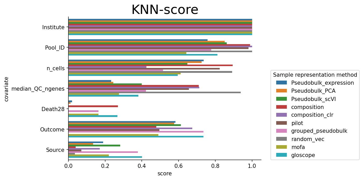
We can see that technical covariates are generally mixed well. For clinically relevant variables, there is some diversity. Let’s now compare outcome trajectory preservation

Evaluation 2 — trajectory preservation

trajectory_results = patpy.tl.trajectory_correlation(
    meta_adata=meta_adata,
    root_sample=root_sample,  # Defined above as the youngest healthy sample
    trajectory_variable="Outcome",
    representations=meta_adata.uns["sample_representations"],
    inverse_trajectory=True,
)
trajectory_results

Diffmap for Pseudobulk_expression already computed, skipping
Diffmap for Pseudobulk_PCA already computed, skipping
Diffmap for Pseudobulk_scVI already computed, skipping
Computing diffmap for composition
Computing diffmap for composition_clr
Computing diffmap for pilot
Computing diffmap for grouped_pseudobulk
Computing diffmap for random_vec
Computing diffmap for mofa
Computing diffmap for gloscope

	correlation
composition_clr	0.716893
Pseudobulk_expression	0.459593
Pseudobulk_PCA	0.450696
pilot	0.418825
gloscope	0.417711
Pseudobulk_scVI	0.400080
grouped_pseudobulk	0.364444
mofa	0.318281
composition	0.244055
random_vec	-0.121616

Let’s now create a clearer visualisation and aggregate all the metrics into 1 score. We compute the total score by weighting batch mixing half as much as trajectory preservation and information retention. The reason is because batch mixing is a very easy task to achieve a high score. If a method doesn’t capture any information (like our random baseline), it achieves a perfect batch mixing score. To make sure methods are prioritised by learning biology, we weigh other scores more:

knn_results_wide = knn_results.pivot(index="representation", columns="covariate", values="score")

# Add trajectory preservation score early so it can feed into col_defs below
knn_results_wide["Trajectory"] = (
    trajectory_results.loc[knn_results_wide.index, "correlation"].abs()
)

# Group covariates by the two scoring buckets, with new display names
display_buckets = {
    "Information retention": benchmark_schema["clinical"].keys(),
    "Batch mixing": benchmark_schema["technical"].keys(),
}

# Per-bucket means -> bucket columns
for bucket, cols in display_buckets.items():
    knn_results_wide[bucket] = knn_results_wide[cols].mean(axis=1)

# New total: (2 * info + 2 * trajectory + batch_mixing) / 5
knn_results_wide["Total"] = (
    2 * knn_results_wide["Information retention"]
    + 2 * knn_results_wide["Trajectory"]
    + knn_results_wide["Batch mixing"]
) / 5

cols_order = ["Total", "Information retention", "Trajectory", "Batch mixing"]
cols_order += display_buckets["Information retention"]
cols_order += display_buckets["Batch mixing"]

cmap_bar = LinearSegmentedColormap.from_list(
    name="bugw", colors=["#FF9693", "#f2fbd2", "#c9ecb4", "#93d3ab", "#35b0ab"], N=256,
)

bar_kw = {
    "cmap": cmap_bar, "plot_bg_bar": True, "annotate": True,
    "height": 0.5, "lw": 0.5, "formatter": lambda x: round(x, 2),
}

col_defs = [
    ColumnDefinition("Total", width=0.7, plot_fn=bar, plot_kw=bar_kw),
    ColumnDefinition(
        "Information retention", width=0.8, plot_fn=bar, plot_kw=bar_kw,
        group="aggregate",
    ),
    ColumnDefinition(
        "Trajectory", width=0.7, plot_fn=bar, plot_kw=bar_kw,
        group="aggregate",
    ),
    ColumnDefinition(
        "Batch mixing", width=0.7, plot_fn=bar, plot_kw=bar_kw,
        group="aggregate",
    ),
]
for col in display_buckets["Information retention"]:
    col_defs.append(ColumnDefinition(
        name=col, width=0.55, formatter=lambda x: round(x, 2),
        textprops={"ha": "center", "bbox": {"boxstyle": "circle", "pad": 0.35}},
        cmap=normed_cmap(knn_results["score"], cmap=matplotlib.cm.PiYG, num_stds=2.5),
        group="Information retention covariates",
    ))
for col in display_buckets["Batch mixing"]:
    col_defs.append(ColumnDefinition(
        name=col, width=0.55, formatter=lambda x: round(x, 2),
        textprops={"ha": "center", "bbox": {"boxstyle": "circle", "pad": 0.35}},
        cmap=normed_cmap(knn_results["score"], cmap=matplotlib.cm.PiYG, num_stds=2.5),
        group="Batch mixing covariates",
    ))

fig, ax = plt.subplots(figsize=(20, 6))
Table(knn_results_wide[cols_order].sort_values("Total", ascending=False), column_definitions=tuple(col_defs), ax=ax)

<plottable.table.Table at 0x7f0ae4a26c50>

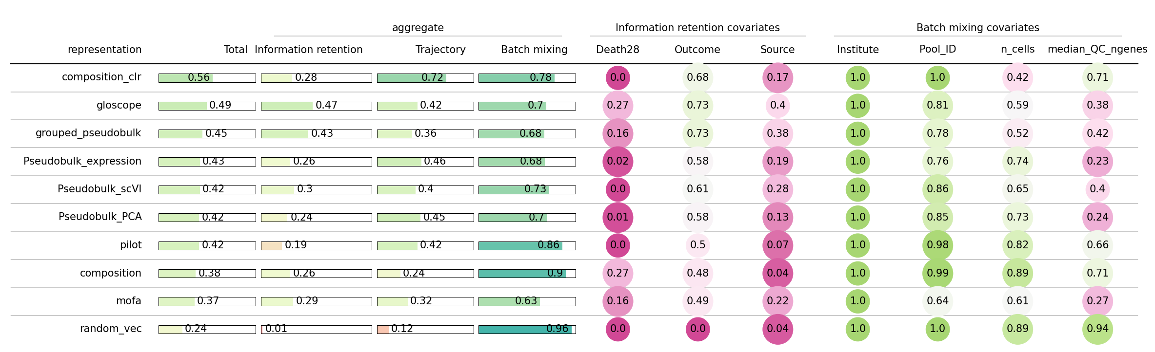
How to read this table

Every cell is a score in [0, 1] where higher = better:

• Clinical columns (Outcome, Death28, Source): high means a kNN classifier trained on the sample distances recovers the clinical label.

• Technical columns (Institute, Pool_ID, n_cells, median_QC_ngenes): high means the opposite — how well the batch effect-related covariates mix.

• trajectory is the absolute Spearman correlation between diffusion pseudotime (rooted at the healthiest donor) and Outcome. High means the order of severity is preserved along the representation’s diffusion graph.

• total is a weighted average that gives more weight to clinical signal than to batch invariance, so the top of the sorted table is the method most useful for downstream clinical analysis on this dataset.

We can see that CLR-transformed composition and GloScope are very good in capturing clinical information. While the former better represents trajectory, the latter better groups different health conditions, and even death in 28 days to some extent. Which method to use depends on the research question.

A reusable benchmark helper

To compare against other datasets we need to repeat the same workflow: run every method, score each one against a “relevant” (clinical) covariate set and a “technical” covariate set, and compute a trajectory correlation. Below is a single helper that does all of that, returning per-method distances, kNN scores, and a summary table. We’ll call it three times: once each for COMBAT (already done above), HLCA, and Stephenson.

import time
import gc
import os

def run_all_methods_on_dataset(
    adata,
    *,
    sample_key,
    cell_type_key,
    layer="X_scVI_batch",
    cluster_size_threshold=5,
    skip_methods=None,
    gloscope_use_gpu=None,
):
    """Run sample-representation methods on `adata`.

    Eight methods total (kept in sync with the COMBAT walkthrough above):
    Pseudobulk on the latent space, CellGroupComposition (raw + CLR),
    PILOT, RandomVector, MOFA, GloScope_py, and GroupedPseudobulk.
    MOFA and GroupedPseudobulk both need a filtered AnnData (cell groups
    with very few cells in some samples make their per-(sample,
    cell_type) aggregations degenerate), so we compute it lazily and
    reuse it.

    Returns
    -------
    dict with keys 'distances', 'samples', 'runtimes' (each keyed by method name).
    """
    out = {"distances": {}, "samples": {}, "runtimes": {}}

    skip_methods = set(skip_methods or [])
    _gloscope_gpu = (
        gloscope_use_gpu if gloscope_use_gpu is not None
        else bool(os.environ.get("PATPY_GLOSCOPE_GPU"))
    )

    adata_filtered = None

    def _ensure_filtered():
        nonlocal adata_filtered
        if adata_filtered is None:
            f = patpy.pp.filter_small_cell_groups(
                adata, sample_key=sample_key, cell_group_key=cell_type_key,
                cluster_size_threshold=cluster_size_threshold,
            )
            # On very wide cohorts (HLCA, OneK1K) the filter can wipe every
            # cell type because few donors have >= threshold cells of *every*
            # type. Fall back to the unfiltered adata in that case so MOFA
            # still has something to fit.
            if f.n_obs == 0:
                print(
                    f"  filter_small_cell_groups(threshold={cluster_size_threshold})"
                    f" removed every cell type; falling back to unfiltered adata"
                )
                f = adata
            adata_filtered = f
        return adata_filtered

    # (method_name, source, factory). `source` selects which adata to fit on:
    # "adata" = the input, "filtered" = small-cell-group-filtered copy.
    method_specs = [
        ("pseudobulk",      "adata",    lambda: patpy.tl.Pseudobulk(
            sample_key=sample_key, cell_group_key=cell_type_key, layer=layer)),
        ("composition",     "adata",    lambda: patpy.tl.CellGroupComposition(
            sample_key=sample_key, cell_group_key=cell_type_key)),
        ("composition_clr", "adata",    lambda: patpy.tl.CellGroupComposition(
            sample_key=sample_key, cell_group_key=cell_type_key, apply_clr=True)),
        ("pilot",           "adata",    lambda: patpy.tl.PILOT(
            sample_key=sample_key, cell_group_key=cell_type_key, layer=layer,
            sample_state_col=sample_key)),  # status is unused for the distance; pass a valid obs column so pilotpy does not KeyError
        ("random_vec",      "adata",    lambda: patpy.tl.RandomVector(
            sample_key=sample_key, cell_group_key=cell_type_key)),
        ("mofa",            "filtered", lambda: patpy.tl.MOFA(
            sample_key=sample_key, cell_group_key=cell_type_key,
            n_factors=10, aggregate_cell_types=True)),
        ("gloscope",        "adata",    lambda: patpy.tl.GloScope_py(
            sample_key=sample_key, cell_group_key=cell_type_key, layer=layer, k=25,
            use_gpu=_gloscope_gpu)),
    ]
    for name, source, factory in method_specs:
        if name in skip_methods:
            print(f"  {name}: skipped")
            continue
        try:
            t0 = time.time()
            m = factory()
            src_adata = _ensure_filtered() if source == "filtered" else adata
            m.prepare_anndata(src_adata)
            out["distances"][name] = m.calculate_distance_matrix(force=True)
            out["samples"][name] = list(m.samples)
            out["runtimes"][name] = time.time() - t0
            print(f"  {name}: {out['runtimes'][name]:.1f}s")
        except Exception as e:
            print(f"  {name} FAILED: {type(e).__name__}: {e}")

    # GroupedPseudobulk also needs the filtered adata.
    if "grouped_pseudobulk" in skip_methods:
        print("  grouped_pseudobulk: skipped")
    else:
        try:
            t0 = time.time()
            m = patpy.tl.GroupedPseudobulk(
                sample_key=sample_key, cell_group_key=cell_type_key, layer=layer)
            m.prepare_anndata(_ensure_filtered())
            out["distances"]["grouped_pseudobulk"] = m.calculate_distance_matrix()
            out["samples"]["grouped_pseudobulk"] = list(m.samples)
            out["runtimes"]["grouped_pseudobulk"] = time.time() - t0
            print(f"  grouped_pseudobulk: {out['runtimes']['grouped_pseudobulk']:.1f}s")
        except Exception as e:
            print(f"  grouped_pseudobulk FAILED: {type(e).__name__}: {e}")

    if adata_filtered is not None:
        del adata_filtered
        gc.collect()

    return out


def score_methods_on_dataset(
    bench_result,
    *,
    metadata,
    sample_key,
    schema,
    root_sample,
    trajectory_variable,
    inverse_trajectory=False,
    n_neighbors=5,
):
    """Score the methods produced by `run_all_methods_on_dataset` against
    a SPARE-style `schema` (dict with at least 'relevant' / 'technical' keys
    mapping to {covariate: task}). Uses `patpy.tl.evaluation.knn_prediction_score`
    -- the same entry point as the COMBAT walkthrough -- and adds a trajectory
    correlation if `trajectory_variable` and `root_sample` are present.

    Returns
    -------
    dict with keys 'long' (long-format scores), 'summary' (per-method
    Information retention / Batch mixing / Trajectory / Runtime / Total),
    and 'meta_adata' (the AnnData used for diffmap).
    """
    methods_all = list(bench_result["distances"].keys())
    # Drop methods that ended up with zero samples (otherwise the
    # intersection across methods is empty and nothing gets scored).
    methods = [m for m in methods_all if len(bench_result["samples"][m]) > 0]
    if len(methods) < len(methods_all):
        empty = [m for m in methods_all if m not in methods]
        print(f"  dropping methods with 0 samples: {empty}")
    method_sample_sets = {m: set(bench_result["samples"][m]) for m in methods}
    common = set.intersection(*method_sample_sets.values()) if method_sample_sets else set()
    common = [s for s in metadata.index if s in common]
    print(f"  scoring on {len(common)} samples (methods: {[(m, len(s)) for m, s in method_sample_sets.items()]})")
    if len(common) < 4:
        print("  too few common samples for kNN scoring; returning empty summary")
        empty = pd.Series(np.nan, index=methods)
        summary = pd.DataFrame({
            "Information retention": empty,
            "Batch mixing": empty,
            "Trajectory": empty,
            "Runtime (s)": pd.Series(bench_result["runtimes"]).reindex(methods),
            "Total": empty,
        })
        return {"long": pd.DataFrame(), "summary": summary, "meta_adata": None}
    meta = metadata.loc[common].copy()
    # Drop all-NaN columns -- ehrapy.encode chokes on them
    meta = meta.dropna(axis=1, how="all")
    meta_adata = ep.io.df_to_anndata(meta)
    meta_adata = ep.pp.encode(meta_adata, autodetect=True)
    # Preserve the raw schema columns on .obs so knn_prediction_score can find
    # them after ep.pp.encode renames the encoded versions.
    for cov_tasks in schema.values():
        for col in cov_tasks:
            if col in meta.columns:
                meta_adata.obs[col] = meta[col].values

    for m in methods:
        order = [bench_result["samples"][m].index(s) for s in common]
        d = bench_result["distances"][m]
        meta_adata.obsm[f"{m}_distances"] = d[np.ix_(order, order)]
        _n_nbrs = min(15, max(2, len(common) - 1))
        ep.pp.neighbors(
            meta_adata, use_rep=f"{m}_distances",
            key_added=f"{m}_neighbors", metric="precomputed",
            n_neighbors=_n_nbrs,
        )
    meta_adata.uns["sample_representations"] = list(methods)

    # KNN scoring via the same patpy entry point used in the COMBAT walkthrough.
    schema_present = {
        group: {col: task for col, task in cov_tasks.items() if col in meta.columns}
        for group, cov_tasks in schema.items()
    }
    long_df = patpy.tl.evaluation.knn_prediction_score(
        meta_adata, schema_present, representations=list(methods),
        n_neighbors=n_neighbors, reverse_technical_score=True,
    )

    # Trajectory correlation
    traj_series = pd.Series(np.nan, index=methods)
    if trajectory_variable in meta.columns and root_sample in meta.index:
        # If trajectory_variable is categorical text, encode to ordered numeric
        traj_target = meta[trajectory_variable]
        if traj_target.dtype.name == "category" or traj_target.dtype == object:
            traj_target_num = traj_target.astype("category").cat.codes.astype(float)
            traj_target_num[traj_target.isna()] = np.nan
            meta_adata.obs[trajectory_variable] = traj_target_num.values
        try:
            traj_df = patpy.tl.trajectory_correlation(
                meta_adata=meta_adata, root_sample=root_sample,
                trajectory_variable=trajectory_variable, representations=methods,
                inverse_trajectory=inverse_trajectory,
            )
            traj_series = traj_df["correlation"].abs()
        except Exception as e:
            print(f"  trajectory_correlation failed: {e}")
    else:
        print(
            f"  trajectory skipped: variable={trajectory_variable!r} in metadata? "
            f"{trajectory_variable in meta.columns}; root={root_sample!r} in samples? "
            f"{root_sample in meta.index}"
        )

    # Per-method summary
    methods_idx = pd.Index(methods, name="representation")
    info = pd.Series({
        m: long_df[
            (long_df["representation"] == m)
            & (long_df["covariate_type"].isin(["relevant", "clinical"]))
        ]["score"].mean()
        for m in methods
    })
    batch = pd.Series({
        m: long_df[
            (long_df["representation"] == m)
            & (long_df["covariate_type"] == "technical")
        ]["score"].mean()
        for m in methods
    })
    traj = traj_series.reindex(methods_idx)
    runtimes_s = pd.Series(bench_result["runtimes"]).reindex(methods_idx)

    summary = pd.DataFrame({
        "Information retention": info,
        "Batch mixing": batch,
        "Trajectory": traj,
        "Runtime (s)": runtimes_s,
    })
    # Total: (2*info + 2*traj + batch) / 5; NaN trajectory falls back to 0 weight
    traj_filled = summary["Trajectory"].fillna(0)
    summary["Total"] = (
        2 * summary["Information retention"].fillna(0)
        + 2 * traj_filled
        + summary["Batch mixing"].fillna(0)
    ) / 5
    summary = summary.sort_values("Total", ascending=False)

    return {"long": long_df, "summary": summary, "meta_adata": meta_adata}

COMBAT summary for the cross-dataset view

# Pre-compute a COMBAT summary in the shape we'll build for HLCA, Stephenson
# and OneK1K. Keep only the scVI pseudobulk variant (the cross-dataset
# helper produces one pseudobulk per dataset) and rename it to match the
# helper's "pseudobulk" key so cross-dataset averaging lines up. The two
# illustrative pseudobulk variants stay in the COMBAT-only table above.
combat_summary = pd.DataFrame({
    "Information retention": knn_results_wide["Information retention"],
    "Batch mixing": knn_results_wide["Batch mixing"],
    "Trajectory": knn_results_wide["Trajectory"],
    "Total": knn_results_wide["Total"],
})
combat_summary = combat_summary.drop(
    ["Pseudobulk_expression", "Pseudobulk_PCA"], errors="ignore"
).rename(index={"Pseudobulk_scVI": "pseudobulk"})
combat_summary["Runtime (s)"] = (
    pd.Series(runtimes["combat"]).reindex(combat_summary.index)
)
combat_summary = combat_summary[
    ["Information retention", "Batch mixing", "Trajectory", "Runtime (s)", "Total"]
]
combat_summary = combat_summary.sort_values("Total", ascending=False)
dataset_summaries["combat"] = combat_summary
combat_summary.round(2)

	Information retention	Batch mixing	Trajectory	Runtime (s)	Total
representation
composition_clr	0.28	0.78	0.72	0.21	0.56
gloscope	0.47	0.70	0.42	246.90	0.49
grouped_pseudobulk	0.43	0.68	0.36	1.05	0.45
pseudobulk	0.30	0.73	0.40	0.30	0.42
pilot	0.19	0.86	0.42	498.57	0.42
composition	0.26	0.90	0.24	0.27	0.38
mofa	0.29	0.63	0.32	15.01	0.37
random_vec	0.01	0.96	0.12	0.01	0.24

# COMBAT analysis done; release the AnnData (and any heavy intermediates) so
# HLCA + Stephenson have memory headroom.
del adata, meta_adata, knn_results, knn_results_wide
gc.collect()

15979

Benchmark on HLCA

On to the Human Lung Cell Atlas (HLCA) []: ~340 donors across health and lung disease, multiple sequencing platforms. We subsample to 50 donors x 20% cells so each method finishes in a few minutes, then run the same seven methods with the SPARE benchmark schema (clinical / technical / trajectory). The summary table at the end is structurally identical to COMBAT’s, just on a different cohort and different question.

hlca, hlca_info = patpy.datasets.hlca(return_dataset_info=True)
print(f"HLCA loaded: {hlca.n_obs} cells, {hlca.obs[hlca_info.sample_key].nunique()} donors")

HLCA loaded: 1687127 cells, 339 donors

hlca = patpy.pp.filter_small_samples(hlca, sample_key=hlca_info.sample_key, sample_size_threshold=200)
print(f'HLCA after QC: {hlca.n_obs} cells, {hlca.obs[hlca_info.sample_key].nunique()} donors')

3 samples removed: homosapiens_None_2023_None_sikkemalisa_002_d10_1101_2022_03_10_483747244C, homosapiens_None_2023_None_sikkemalisa_002_d10_1101_2022_03_10_483747NP11, homosapiens_None_2023_None_sikkemalisa_002_d10_1101_2022_03_10_483747VUHD105
HLCA after QC: 1686679 cells, 336 donors

# Extract sample-level metadata for the SPARE-style scoring (clinical = "relevant",
# technical = batch / acquisition artefacts). Skip "contextual" columns -- we don't
# score them, they're neither clinical signal nor technical noise.
hlca_sample_cols = [
    "tissue", "anatomical_region_ccf_score", "lung_condition", "disease",
    "smoking_status", "suspension_type", "core_or_extension", "fresh_or_frozen",
    "sequencing_platform", "subject_type", "assay", "development_stage",
    "BMI", "age_or_mean_of_age_range", "sex",
]
# Only ask for columns that exist
hlca_sample_cols = [c for c in hlca_sample_cols if c in hlca.obs.columns]
hlca_meta = patpy.pp.extract_metadata(hlca, hlca_info.sample_key, hlca_sample_cols)
hlca_qc = patpy.pp.calculate_cell_qc_metrics(
    hlca, sample_key=hlca_info.sample_key,
    cell_qc_vars=[c for c in ["n_genes_by_counts", "total_counts", "pct_counts_mt"] if c in hlca.obs.columns],
)
hlca_ncells = patpy.pp.calculate_n_cells_per_sample(hlca, hlca_info.sample_key)
hlca_meta = pd.concat([hlca_meta, hlca_qc.loc[hlca_meta.index], hlca_ncells.loc[hlca_meta.index]], axis=1)
hlca_meta.head()

	tissue	anatomical_region_ccf_score	lung_condition	disease	smoking_status	suspension_type	core_or_extension	fresh_or_frozen	sequencing_platform	subject_type	assay	development_stage	BMI	age_or_mean_of_age_range	sex	median_n_genes_by_counts	median_total_counts	median_pct_counts_mt	n_cells
donor_id
homosapiens_None_2023_None_sikkemalisa_002_d10_1101_2022_03_10_483747Donor_02	lung parenchyma	0.97	Healthy	normal	former	cell	core	fresh	Illumina HiSeq 4000	organ_donor	10x 3' v2	55-year-old stage	NaN	55.0	male	204.0	330.554077	0.0	3832
homosapiens_None_2023_None_sikkemalisa_002_d10_1101_2022_03_10_483747cc05p	lung	NaN	Healthy	normal	NaN	cell	extension	NaN	NaN	NaN	10x 3' v2	unknown	NaN	NaN	unknown	145.0	301.329895	0.0	1687
homosapiens_None_2023_None_sikkemalisa_002_d10_1101_2022_03_10_483747VUHD68	lung parenchyma	0.97	Healthy	normal	former	cell	core	fresh	Illumina NovaSeq 6000 S1	organ_donor	10x 5' v1	41-year-old stage	23.5	41.0	male	183.0	344.931091	0.0	7850
homosapiens_None_2023_None_sikkemalisa_002_d10_1101_2022_03_10_483747D062	lung	NaN	Healthy	normal	NaN	nucleus	extension	NaN	NaN	NaN	10x 3' v3	newborn stage (0-28 days)	NaN	0.0	male	135.0	231.189117	0.0	4852
homosapiens_None_2023_None_sikkemalisa_002_d10_1101_2022_03_10_483747donor 1	lung parenchyma	0.97	Healthy (tumor adjacent)	normal	former	cell	core	fresh	Illumina NovaSeq 6000	alive_disease	10x 3' v2	75-year-old stage	24.6	75.0	male	197.0	338.632477	0.0	7523

print("Running methods on HLCA (skip GroupedPseudobulk -- per-cell-type filter\n"
      "     wipes too many sparse cell types; CPU GloScope -- cuml OOMs on V100\n"
      "     with 1.7M cells):")
hlca_bench = run_all_methods_on_dataset(
    hlca,
    sample_key=hlca_info.sample_key,
    cell_type_key=hlca_info.cell_type_key,
    layer="X_scVI_batch",
    skip_methods=["grouped_pseudobulk"],
    gloscope_use_gpu=True  # A100 GPU is fast enough on the new env,
)
runtimes["hlca"] = hlca_bench["runtimes"]

Running methods on HLCA (skip GroupedPseudobulk -- per-cell-type filter
     wipes too many sparse cell types; CPU GloScope -- cuml OOMs on V100
     with 1.7M cells):
  pseudobulk: 1.8s
  composition: 7.0s
  composition_clr: 0.7s
  pilot: 31.8s
  random_vec: 0.0s
51 cell types removed: alveolar type 1 fibroblast cell, non-classical monocyte, smooth muscle cell, ionocyte, B cell, club cell, hematopoietic stem cell, pulmonary alveolar type 1 cell, mast cell, bronchial goblet cell, lung pericyte, ciliated columnar cell of tracheobronchial tree, alveolar adventitial fibroblast, respiratory basal cell, serous secreting cell, endothelial cell of lymphatic vessel, brush cell of tracheobronchial tree, fibroblast, capillary endothelial cell, lung neuroendocrine cell, classical monocyte, plasma cell, acinar cell, CD8-positive, alpha-beta T cell, vein endothelial cell, tracheobronchial goblet cell, conventional dendritic cell, tracheobronchial serous cell, pulmonary artery endothelial cell, elicited macrophage, alveolar macrophage, stromal cell, respiratory hillock cell, CD4-positive, alpha-beta T cell, epithelial cell of alveolus of lung, pulmonary alveolar type 2 cell, natural killer cell, tracheobronchial smooth muscle cell, bronchus fibroblast of lung, mesothelial cell, mucus secreting cell, T cell, unknown, lung macrophage, plasmacytoid dendritic cell, epithelial cell of lower respiratory tract, CD1c-positive myeloid dendritic cell, nasal mucosa goblet cell, myofibroblast cell, dendritic cell, multi-ciliated epithelial cell
  filter_small_cell_groups(threshold=5) removed every cell type; falling back to unfiltered adata

        #########################################################
        ###           __  __  ____  ______                    ### 
        ###          |  \/  |/ __ \|  ____/\    _             ### 
        ###          | \  / | |  | | |__ /  \ _| |_           ### 
        ###          | |\/| | |  | |  __/ /\ \_   _|          ###
        ###          | |  | | |__| | | / ____ \|_|            ###
        ###          |_|  |_|\____/|_|/_/    \_\              ###
        ###                                                   ### 
        #########################################################
Features names not provided, using default naming convention:
- feature1_view1, featureD_viewM

Successfully loaded view='alveolar macrophage' group='group1' with N=336 samples and D=3000 features...
Successfully loaded view='unknown' group='group1' with N=336 samples and D=3000 features...
Successfully loaded view='capillary endothelial cell' group='group1' with N=336 samples and D=3000 features...
Successfully loaded view='alveolar type 1 fibroblast cell' group='group1' with N=336 samples and D=3000 features...
Successfully loaded view='pulmonary artery endothelial cell' group='group1' with N=336 samples and D=3000 features...
Successfully loaded view='nasal mucosa goblet cell' group='group1' with N=336 samples and D=3000 features...
Successfully loaded view='CD8-positive, alpha-beta T cell' group='group1' with N=336 samples and D=3000 features...
Successfully loaded view='club cell' group='group1' with N=336 samples and D=3000 features...
Successfully loaded view='respiratory hillock cell' group='group1' with N=336 samples and D=3000 features...
Successfully loaded view='B cell' group='group1' with N=336 samples and D=3000 features...
Successfully loaded view='alveolar adventitial fibroblast' group='group1' with N=336 samples and D=3000 features...
Successfully loaded view='lung pericyte' group='group1' with N=336 samples and D=3000 features...
Successfully loaded view='elicited macrophage' group='group1' with N=336 samples and D=3000 features...
Successfully loaded view='classical monocyte' group='group1' with N=336 samples and D=3000 features...
Successfully loaded view='mast cell' group='group1' with N=336 samples and D=3000 features...
Successfully loaded view='endothelial cell of lymphatic vessel' group='group1' with N=336 samples and D=3000 features...
Successfully loaded view='respiratory basal cell' group='group1' with N=336 samples and D=3000 features...
Successfully loaded view='CD1c-positive myeloid dendritic cell' group='group1' with N=336 samples and D=3000 features...
Successfully loaded view='pulmonary alveolar type 2 cell' group='group1' with N=336 samples and D=3000 features...
Successfully loaded view='ciliated columnar cell of tracheobronchial tree' group='group1' with N=336 samples and D=3000 features...
Successfully loaded view='natural killer cell' group='group1' with N=336 samples and D=3000 features...
Successfully loaded view='tracheobronchial serous cell' group='group1' with N=336 samples and D=3000 features...
Successfully loaded view='CD4-positive, alpha-beta T cell' group='group1' with N=336 samples and D=3000 features...
Successfully loaded view='pulmonary alveolar type 1 cell' group='group1' with N=336 samples and D=3000 features...
Successfully loaded view='myofibroblast cell' group='group1' with N=336 samples and D=3000 features...
Successfully loaded view='mucus secreting cell' group='group1' with N=336 samples and D=3000 features...
Successfully loaded view='lung macrophage' group='group1' with N=336 samples and D=3000 features...
Successfully loaded view='non-classical monocyte' group='group1' with N=336 samples and D=3000 features...
Successfully loaded view='smooth muscle cell' group='group1' with N=336 samples and D=3000 features...
Successfully loaded view='epithelial cell of lower respiratory tract' group='group1' with N=336 samples and D=3000 features...
Successfully loaded view='epithelial cell of alveolus of lung' group='group1' with N=336 samples and D=3000 features...
Successfully loaded view='vein endothelial cell' group='group1' with N=336 samples and D=3000 features...
Successfully loaded view='T cell' group='group1' with N=336 samples and D=3000 features...
Successfully loaded view='multi-ciliated epithelial cell' group='group1' with N=336 samples and D=3000 features...
Successfully loaded view='ionocyte' group='group1' with N=336 samples and D=3000 features...
Successfully loaded view='tracheobronchial smooth muscle cell' group='group1' with N=336 samples and D=3000 features...
Successfully loaded view='plasma cell' group='group1' with N=336 samples and D=3000 features...
Successfully loaded view='conventional dendritic cell' group='group1' with N=336 samples and D=3000 features...
Successfully loaded view='bronchus fibroblast of lung' group='group1' with N=336 samples and D=3000 features...
Successfully loaded view='plasmacytoid dendritic cell' group='group1' with N=336 samples and D=3000 features...
Successfully loaded view='stromal cell' group='group1' with N=336 samples and D=3000 features...
Successfully loaded view='serous secreting cell' group='group1' with N=336 samples and D=3000 features...
Successfully loaded view='lung neuroendocrine cell' group='group1' with N=336 samples and D=3000 features...
Successfully loaded view='fibroblast' group='group1' with N=336 samples and D=3000 features...
Successfully loaded view='bronchial goblet cell' group='group1' with N=336 samples and D=3000 features...
Successfully loaded view='acinar cell' group='group1' with N=336 samples and D=3000 features...
Successfully loaded view='dendritic cell' group='group1' with N=336 samples and D=3000 features...
Successfully loaded view='tracheobronchial goblet cell' group='group1' with N=336 samples and D=3000 features...
Successfully loaded view='mesothelial cell' group='group1' with N=336 samples and D=3000 features...
Successfully loaded view='brush cell of tracheobronchial tree' group='group1' with N=336 samples and D=3000 features...
Successfully loaded view='hematopoietic stem cell' group='group1' with N=336 samples and D=3000 features...
Model options:
- Automatic Relevance Determination prior on the factors: False
- Automatic Relevance Determination prior on the weights: True
- Spike-and-slab prior on the factors: False
- Spike-and-slab prior on the weights: True
Likelihoods:
- View 0 (alveolar macrophage): gaussian
- View 1 (unknown): gaussian
- View 2 (capillary endothelial cell): gaussian
- View 3 (alveolar type 1 fibroblast cell): gaussian
- View 4 (pulmonary artery endothelial cell): gaussian
- View 5 (nasal mucosa goblet cell): gaussian
- View 6 (CD8-positive, alpha-beta T cell): gaussian
- View 7 (club cell): gaussian
- View 8 (respiratory hillock cell): gaussian
- View 9 (B cell): gaussian
- View 10 (alveolar adventitial fibroblast): gaussian
- View 11 (lung pericyte): gaussian
- View 12 (elicited macrophage): gaussian
- View 13 (classical monocyte): gaussian
- View 14 (mast cell): gaussian
- View 15 (endothelial cell of lymphatic vessel): gaussian
- View 16 (respiratory basal cell): gaussian
- View 17 (CD1c-positive myeloid dendritic cell): gaussian
- View 18 (pulmonary alveolar type 2 cell): gaussian
- View 19 (ciliated columnar cell of tracheobronchial tree): gaussian
- View 20 (natural killer cell): gaussian
- View 21 (tracheobronchial serous cell): gaussian
- View 22 (CD4-positive, alpha-beta T cell): gaussian
- View 23 (pulmonary alveolar type 1 cell): gaussian
- View 24 (myofibroblast cell): gaussian
- View 25 (mucus secreting cell): gaussian
- View 26 (lung macrophage): gaussian
- View 27 (non-classical monocyte): gaussian
- View 28 (smooth muscle cell): gaussian
- View 29 (epithelial cell of lower respiratory tract): gaussian
- View 30 (epithelial cell of alveolus of lung): gaussian
- View 31 (vein endothelial cell): gaussian
- View 32 (T cell): gaussian
- View 33 (multi-ciliated epithelial cell): gaussian
- View 34 (ionocyte): gaussian
- View 35 (tracheobronchial smooth muscle cell): gaussian
- View 36 (plasma cell): gaussian
- View 37 (conventional dendritic cell): gaussian
- View 38 (bronchus fibroblast of lung): gaussian
- View 39 (plasmacytoid dendritic cell): gaussian
- View 40 (stromal cell): gaussian
- View 41 (serous secreting cell): gaussian
- View 42 (lung neuroendocrine cell): gaussian
- View 43 (fibroblast): gaussian
- View 44 (bronchial goblet cell): gaussian
- View 45 (acinar cell): gaussian
- View 46 (dendritic cell): gaussian
- View 47 (tracheobronchial goblet cell): gaussian
- View 48 (mesothelial cell): gaussian
- View 49 (brush cell of tracheobronchial tree): gaussian
- View 50 (hematopoietic stem cell): gaussian


######################################
## Training the model with seed 67 ##
######################################
ELBO before training: -174422174.12
Iteration 1: time=2.22, ELBO=24582147.79, deltaELBO=199004321.906 (114.09347631%), Factors=10
Iteration 2: time=1.69, ELBO=47648875.21, deltaELBO=23066727.429 (13.22465308%), Factors=10
Iteration 3: time=1.70, ELBO=48384578.06, deltaELBO=735702.850 (0.42179434%), Factors=10
Iteration 4: time=1.71, ELBO=48533717.55, deltaELBO=149139.488 (0.08550489%), Factors=10
Iteration 5: time=1.71, ELBO=48663689.61, deltaELBO=129972.053 (0.07451579%), Factors=10
Iteration 6: time=1.76, ELBO=48773840.44, deltaELBO=110150.838 (0.06315185%), Factors=10
Iteration 7: time=1.78, ELBO=48855440.24, deltaELBO=81599.796 (0.04678293%), Factors=10
Iteration 8: time=1.80, ELBO=48922773.66, deltaELBO=67333.418 (0.03860370%), Factors=10
Iteration 9: time=1.84, ELBO=48984749.50, deltaELBO=61975.844 (0.03553209%), Factors=10
Iteration 10: time=1.83, ELBO=49042994.50, deltaELBO=58245.004 (0.03339312%), Factors=10
Iteration 11: time=1.84, ELBO=49098031.59, deltaELBO=55037.081 (0.03155395%), Factors=10
Iteration 12: time=1.82, ELBO=49149823.30, deltaELBO=51791.717 (0.02969331%), Factors=10
Iteration 13: time=1.83, ELBO=49200393.95, deltaELBO=50570.648 (0.02899325%), Factors=10
Iteration 14: time=1.82, ELBO=49251905.22, deltaELBO=51511.268 (0.02953252%), Factors=10
Iteration 15: time=1.82, ELBO=49301715.89, deltaELBO=49810.670 (0.02855753%), Factors=10
Iteration 16: time=1.83, ELBO=49348359.25, deltaELBO=46643.361 (0.02674165%), Factors=10
Iteration 17: time=1.84, ELBO=49390422.63, deltaELBO=42063.382 (0.02411585%), Factors=10
Iteration 18: time=1.83, ELBO=49427587.22, deltaELBO=37164.582 (0.02130726%), Factors=10
Iteration 19: time=1.83, ELBO=49459699.32, deltaELBO=32112.107 (0.01841056%), Factors=10
Iteration 20: time=1.83, ELBO=49487921.55, deltaELBO=28222.227 (0.01618041%), Factors=10
Iteration 21: time=1.82, ELBO=49513518.18, deltaELBO=25596.626 (0.01467510%), Factors=10
Iteration 22: time=1.80, ELBO=49537211.10, deltaELBO=23692.926 (0.01358367%), Factors=10
Iteration 23: time=1.84, ELBO=49559247.31, deltaELBO=22036.212 (0.01263384%), Factors=10
Iteration 24: time=1.82, ELBO=49580084.33, deltaELBO=20837.015 (0.01194631%), Factors=10
Iteration 25: time=1.84, ELBO=49600664.73, deltaELBO=20580.397 (0.01179919%), Factors=10
Iteration 26: time=1.84, ELBO=49620599.00, deltaELBO=19934.279 (0.01142875%), Factors=10
Iteration 27: time=1.85, ELBO=49638889.61, deltaELBO=18290.605 (0.01048640%), Factors=10
Iteration 28: time=1.84, ELBO=49655572.67, deltaELBO=16683.064 (0.00956476%), Factors=10
Iteration 29: time=1.82, ELBO=49671071.49, deltaELBO=15498.818 (0.00888581%), Factors=10
Iteration 30: time=1.85, ELBO=49685374.19, deltaELBO=14302.698 (0.00820005%), Factors=10
Iteration 31: time=2.74, ELBO=49698924.47, deltaELBO=13550.280 (0.00776867%), Factors=10
Iteration 32: time=2.21, ELBO=49712068.11, deltaELBO=13143.641 (0.00753553%), Factors=10
Iteration 33: time=1.84, ELBO=49724601.18, deltaELBO=12533.071 (0.00718548%), Factors=10
Iteration 34: time=1.82, ELBO=49736423.09, deltaELBO=11821.905 (0.00677775%), Factors=10
Iteration 35: time=1.83, ELBO=49747537.61, deltaELBO=11114.522 (0.00637220%), Factors=10
Iteration 36: time=1.81, ELBO=49758056.65, deltaELBO=10519.039 (0.00603079%), Factors=10
Iteration 37: time=1.84, ELBO=49768089.35, deltaELBO=10032.707 (0.00575197%), Factors=10
Iteration 38: time=1.85, ELBO=49777602.57, deltaELBO=9513.215 (0.00545413%), Factors=10
Iteration 39: time=1.85, ELBO=49786576.21, deltaELBO=8973.642 (0.00514478%), Factors=10
Iteration 40: time=1.85, ELBO=49794908.12, deltaELBO=8331.910 (0.00477686%), Factors=10
Iteration 41: time=2.13, ELBO=49802625.52, deltaELBO=7717.397 (0.00442455%), Factors=10
Iteration 42: time=1.87, ELBO=49809982.93, deltaELBO=7357.411 (0.00421816%), Factors=10
Iteration 43: time=1.82, ELBO=49817074.82, deltaELBO=7091.886 (0.00406593%), Factors=10
Iteration 44: time=1.88, ELBO=49823925.24, deltaELBO=6850.428 (0.00392750%), Factors=10
Iteration 45: time=1.85, ELBO=49830520.72, deltaELBO=6595.477 (0.00378133%), Factors=10
Iteration 46: time=1.85, ELBO=49836809.51, deltaELBO=6288.792 (0.00360550%), Factors=10
Iteration 47: time=1.83, ELBO=49842690.63, deltaELBO=5881.112 (0.00337177%), Factors=10
Iteration 48: time=1.85, ELBO=49848083.37, deltaELBO=5392.744 (0.00309178%), Factors=10
Iteration 49: time=1.85, ELBO=49853071.82, deltaELBO=4988.453 (0.00285999%), Factors=10
Iteration 50: time=1.82, ELBO=50627555.89, deltaELBO=774484.067 (0.44402844%), Factors=10
Iteration 51: time=1.85, ELBO=50791562.95, deltaELBO=164007.064 (0.09402879%), Factors=10
Iteration 52: time=1.90, ELBO=50823076.18, deltaELBO=31513.225 (0.01806721%), Factors=10
Iteration 53: time=1.77, ELBO=50833474.40, deltaELBO=10398.217 (0.00596152%), Factors=10
Iteration 54: time=1.77, ELBO=50839114.31, deltaELBO=5639.914 (0.00323348%), Factors=10
Iteration 55: time=1.84, ELBO=50843240.91, deltaELBO=4126.596 (0.00236587%), Factors=10
Iteration 56: time=1.84, ELBO=50846808.75, deltaELBO=3567.844 (0.00204552%), Factors=10
Iteration 57: time=1.81, ELBO=50849968.95, deltaELBO=3160.204 (0.00181181%), Factors=10
Iteration 58: time=1.85, ELBO=50852663.04, deltaELBO=2694.084 (0.00154458%), Factors=10
Iteration 59: time=1.86, ELBO=50854986.53, deltaELBO=2323.495 (0.00133211%), Factors=10
Iteration 60: time=1.87, ELBO=50857049.00, deltaELBO=2062.467 (0.00118246%), Factors=10
Iteration 61: time=1.82, ELBO=50859034.54, deltaELBO=1985.539 (0.00113835%), Factors=10
Iteration 62: time=1.89, ELBO=50860789.68, deltaELBO=1755.144 (0.00100626%), Factors=10
Iteration 63: time=1.82, ELBO=50862438.43, deltaELBO=1648.751 (0.00094526%), Factors=10
Iteration 64: time=1.80, ELBO=50863991.45, deltaELBO=1553.020 (0.00089038%), Factors=10
Iteration 65: time=2.20, ELBO=50865471.85, deltaELBO=1480.393 (0.00084874%), Factors=10
Iteration 66: time=1.94, ELBO=50866887.72, deltaELBO=1415.870 (0.00081175%), Factors=10
Iteration 67: time=1.85, ELBO=50868245.95, deltaELBO=1358.234 (0.00077870%), Factors=10
Iteration 68: time=1.85, ELBO=50869561.37, deltaELBO=1315.420 (0.00075416%), Factors=10
Iteration 69: time=1.85, ELBO=50870840.05, deltaELBO=1278.680 (0.00073309%), Factors=10
Iteration 70: time=1.84, ELBO=50872071.81, deltaELBO=1231.764 (0.00070620%), Factors=10
Iteration 71: time=1.82, ELBO=50873283.62, deltaELBO=1211.802 (0.00069475%), Factors=10
Iteration 72: time=1.85, ELBO=50874488.31, deltaELBO=1204.694 (0.00069068%), Factors=10
Iteration 73: time=1.85, ELBO=50875658.95, deltaELBO=1170.640 (0.00067115%), Factors=10
Iteration 74: time=1.85, ELBO=50876799.81, deltaELBO=1140.859 (0.00065408%), Factors=10
Iteration 75: time=1.82, ELBO=50877920.05, deltaELBO=1120.240 (0.00064226%), Factors=10
Iteration 76: time=1.82, ELBO=50879016.32, deltaELBO=1096.269 (0.00062851%), Factors=10
Iteration 77: time=1.86, ELBO=50880102.91, deltaELBO=1086.591 (0.00062297%), Factors=10
Iteration 78: time=1.74, ELBO=50881171.29, deltaELBO=1068.385 (0.00061253%), Factors=10
Iteration 79: time=1.84, ELBO=50882228.86, deltaELBO=1057.569 (0.00060633%), Factors=10
Iteration 80: time=1.84, ELBO=50883305.69, deltaELBO=1076.828 (0.00061737%), Factors=10
Iteration 81: time=1.84, ELBO=50884326.36, deltaELBO=1020.664 (0.00058517%), Factors=10
Iteration 82: time=1.83, ELBO=50885332.60, deltaELBO=1006.248 (0.00057690%), Factors=10
Iteration 83: time=1.82, ELBO=50886335.68, deltaELBO=1003.077 (0.00057509%), Factors=10
Iteration 84: time=1.84, ELBO=50887335.68, deltaELBO=999.999 (0.00057332%), Factors=10
Iteration 85: time=1.80, ELBO=50888306.25, deltaELBO=970.574 (0.00055645%), Factors=10
Iteration 86: time=1.85, ELBO=50889243.49, deltaELBO=937.236 (0.00053734%), Factors=10
Iteration 87: time=1.85, ELBO=50890176.37, deltaELBO=932.881 (0.00053484%), Factors=10
Iteration 88: time=1.85, ELBO=50891082.70, deltaELBO=906.327 (0.00051962%), Factors=10
Iteration 89: time=1.84, ELBO=50891984.12, deltaELBO=901.426 (0.00051681%), Factors=10
Iteration 90: time=1.85, ELBO=50892916.76, deltaELBO=932.634 (0.00053470%), Factors=10
Iteration 91: time=1.85, ELBO=50893854.08, deltaELBO=937.326 (0.00053739%), Factors=10
Iteration 92: time=1.82, ELBO=50894770.87, deltaELBO=916.785 (0.00052561%), Factors=10
Iteration 93: time=1.85, ELBO=50895654.18, deltaELBO=883.310 (0.00050642%), Factors=10
Iteration 94: time=1.86, ELBO=50896515.67, deltaELBO=861.492 (0.00049391%), Factors=10
Iteration 95: time=1.83, ELBO=50897382.43, deltaELBO=866.758 (0.00049693%), Factors=10

Converged!



#######################
## Training finished ##
#######################
  mofa: 550.6s
  gloscope: 205.6s
  grouped_pseudobulk: skipped

# SPARE schema for HLCA (https://github.com/lueckenlab/SPARE/blob/main/data/hlca/benchmark_schema.json)
hlca_schema = {
    "relevant": {
        "tissue": "classification",
        "anatomical_region_ccf_score": "regression",
        "lung_condition": "classification",
        "disease": "classification",
        "smoking_status": "classification",
    },
    "technical": {
        "suspension_type": "classification",
        "core_or_extension": "classification",
        "fresh_or_frozen": "classification",
        "sequencing_platform": "classification",
        "subject_type": "classification",
        "assay": "classification",
        "median_n_genes_by_counts": "regression",
        "median_total_counts": "regression",
        "median_pct_counts_mt": "regression",
        "n_cells": "regression",
        "development_stage": "classification",
    },
}

hlca_scored = score_methods_on_dataset(
    hlca_bench,
    metadata=hlca_meta,
    sample_key=hlca_info.sample_key,
    schema=hlca_schema,
    root_sample="homosapiens_None_2023_None_sikkemalisa_002_d10_1101_2022_03_10_483747D322",
    trajectory_variable="anatomical_region_ccf_score",
    inverse_trajectory=False,
)
dataset_summaries["hlca"] = hlca_scored["summary"]
hlca_scored["summary"].round(2)

  scoring on 336 samples (methods: [('pseudobulk', 336), ('composition', 336), ('composition_clr', 336), ('pilot', 336), ('random_vec', 336), ('mofa', 336), ('gloscope', 336)])
! Feature 'median_pct_counts_mt' was detected as categorical features stored numerically.Please verify and correct using `ep.ad.replace_feature_types` if necessary.
! Feature types were inferred and stored in adata.var[feature_type]. Please verify using `ep.ad.feature_type_overview` and adjust if necessary using `ep.ad.replace_feature_types`.
Computing diffmap for pseudobulk
Computing diffmap for composition
Computing diffmap for composition_clr
Computing diffmap for pilot
Computing diffmap for random_vec
Computing diffmap for mofa
Computing diffmap for gloscope

	Information retention	Batch mixing	Trajectory	Runtime (s)	Total
composition_clr	0.55	0.36	0.81	0.69	0.61
pseudobulk	0.53	0.38	0.81	1.84	0.61
gloscope	0.58	0.33	0.76	205.63	0.60
pilot	0.47	0.46	0.80	31.82	0.60
composition	0.45	0.47	0.40	6.98	0.43
mofa	0.36	0.52	0.45	550.62	0.43
random_vec	0.00	0.99	0.08	0.02	0.23

# Free HLCA to keep peak memory low before Stephenson loads
del hlca, hlca_bench, hlca_scored
gc.collect()

9

Benchmark on Stephenson

A third cohort to show the workflow generalises beyond two datasets. Stephenson et al. [] is another COVID-19 PBMC study, with 131 donors collected across three UK sites – so a different clinical schema (Worst_Clinical_Status, Status_on_day_collection_summary) and a different technical artefact (Site).

stephenson, stephenson_info = patpy.datasets.stephenson(return_dataset_info=True)
print(f'Stephenson: {stephenson.n_obs} cells, {stephenson.obs[stephenson_info.sample_key].nunique()} donors')

Stephenson: 639482 cells, 131 donors

stephenson_sample_cols = [
    "Status", "Status_on_day_collection_summary", "Days_from_onset",
    "Worst_Clinical_Status", "Outcome", "disease", "Site",
    "Swab_result", "Smoker", "sex", "development_stage",
]
stephenson_sample_cols = [c for c in stephenson_sample_cols if c in stephenson.obs.columns]
stephenson = patpy.pp.filter_small_samples(stephenson, sample_key=stephenson_info.sample_key, sample_size_threshold=200)
stephenson_meta = patpy.pp.extract_metadata(stephenson, stephenson_info.sample_key, stephenson_sample_cols)
stephenson_qc = patpy.pp.calculate_cell_qc_metrics(
    stephenson, sample_key=stephenson_info.sample_key,
    cell_qc_vars=[c for c in ["n_genes_by_counts", "total_counts", "pct_counts_mt"] if c in stephenson.obs.columns],
)
stephenson_ncells = patpy.pp.calculate_n_cells_per_sample(stephenson, stephenson_info.sample_key)
stephenson_meta = pd.concat(
    [stephenson_meta, stephenson_qc.loc[stephenson_meta.index], stephenson_ncells.loc[stephenson_meta.index]],
    axis=1,
)
print(f"Stephenson metadata shape: {stephenson_meta.shape}")

0 samples removed:
Stephenson metadata shape: (131, 15)

print("Running 7 methods on Stephenson:")
stephenson_bench = run_all_methods_on_dataset(
    stephenson,
    sample_key=stephenson_info.sample_key,
    cell_type_key=stephenson_info.cell_type_key,
    layer="X_scVI_batch",
)
runtimes["stephenson"] = stephenson_bench["runtimes"]

Running 7 methods on Stephenson:
  pseudobulk: 0.3s
  composition: 0.5s
  composition_clr: 0.2s
  pilot: 5.5s
  random_vec: 0.0s
45 cell types removed: naive thymus-derived CD4-positive, alpha-beta T cell, effector memory CD4-positive, alpha-beta T cell, group 2 innate lymphoid cell, human, erythrocyte, B cell, CD14-low, CD16-positive monocyte, CD34-positive, CD38-negative hematopoietic stem cell, CD14-positive monocyte, malignant cell, dendritic cell, human, erythroid progenitor cell, mammalian, IgM plasma cell, effector memory CD8-positive, alpha-beta T cell, T follicular helper cell, T-helper 2 cell, T-helper 22 cell, IgA plasma cell, unswitched memory B cell, CD8-positive, alpha-beta T cell, megakaryocyte, myeloid dendritic cell, myeloid lineage restricted progenitor cell, gamma-delta T cell, class switched memory B cell, regulatory T cell, CD16-negative, CD56-bright natural killer cell, human, CD4-positive, alpha-beta T cell, ILC1, human, T-helper 17 cell, natural killer cell, hematopoietic precursor cell, mucosal invariant T cell, naive thymus-derived CD8-positive, alpha-beta T cell, platelet, IgG plasma cell, effector CD8-positive, alpha-beta T cell, central memory CD4-positive, alpha-beta T cell, immature B cell, plasmablast, plasmacytoid dendritic cell, naive B cell, monocyte, T-helper 1 cell, dendritic cell, mature NK T cell

        #########################################################
        ###           __  __  ____  ______                    ### 
        ###          |  \/  |/ __ \|  ____/\    _             ### 
        ###          | \  / | |  | | |__ /  \ _| |_           ### 
        ###          | |\/| | |  | |  __/ /\ \_   _|          ###
        ###          | |  | | |__| | | / ____ \|_|            ###
        ###          |_|  |_|\____/|_|/_/    \_\              ###
        ###                                                   ### 
        #########################################################
Features names not provided, using default naming convention:
- feature1_view1, featureD_viewM

Successfully loaded view='CD16-positive, CD56-dim natural killer cell, human' group='group1' with N=131 samples and D=3000 features...


Warning: 401 features(s) in view 0 have zero variance, consider removing them before training the model...
Model options:
- Automatic Relevance Determination prior on the factors: False
- Automatic Relevance Determination prior on the weights: True
- Spike-and-slab prior on the factors: False
- Spike-and-slab prior on the weights: True
Likelihoods:
- View 0 (CD16-positive, CD56-dim natural killer cell, human): gaussian


######################################
## Training the model with seed 67 ##
######################################


ELBO before training: -2866357.76 

Iteration 1: time=0.07, ELBO=532587.83, deltaELBO=3398945.591 (118.58064734%), Factors=10
Iteration 2: time=0.02, ELBO=1175000.37, deltaELBO=642412.546 (22.41215503%), Factors=10
Iteration 3: time=0.03, ELBO=1189341.61, deltaELBO=14341.242 (0.50032979%), Factors=10
Iteration 4: time=0.02, ELBO=1191813.15, deltaELBO=2471.539 (0.08622575%), Factors=10
Iteration 5: time=0.02, ELBO=1193608.28, deltaELBO=1795.130 (0.06262755%), Factors=10
Iteration 6: time=0.02, ELBO=1193866.42, deltaELBO=258.135 (0.00900567%), Factors=10
Iteration 7: time=0.02, ELBO=1194025.14, deltaELBO=158.721 (0.00553737%), Factors=10
Iteration 8: time=0.02, ELBO=1194158.16, deltaELBO=133.023 (0.00464083%), Factors=10
Iteration 9: time=0.02, ELBO=1194278.47, deltaELBO=120.313 (0.00419742%), Factors=10
Iteration 10: time=0.02, ELBO=1194389.85, deltaELBO=111.380 (0.00388575%), Factors=10
Iteration 11: time=0.02, ELBO=1194495.76, deltaELBO=105.902 (0.00369464%), Factors=10
Iteration 12: time=0.02, ELBO=1194598.62, deltaELBO=102.867 (0.00358876%), Factors=10
Iteration 13: time=0.02, ELBO=1194698.82, deltaELBO=100.198 (0.00349567%), Factors=10
Iteration 14: time=0.02, ELBO=1194795.84, deltaELBO=97.024 (0.00338492%), Factors=10
Iteration 15: time=0.02, ELBO=1194890.08, deltaELBO=94.230 (0.00328746%), Factors=10
Iteration 16: time=0.02, ELBO=1194982.31, deltaELBO=92.238 (0.00321795%), Factors=10
Iteration 17: time=0.02, ELBO=1195073.25, deltaELBO=90.932 (0.00317239%), Factors=10
Iteration 18: time=0.02, ELBO=1195163.32, deltaELBO=90.075 (0.00314250%), Factors=10
Iteration 19: time=0.02, ELBO=1195252.74, deltaELBO=89.422 (0.00311972%), Factors=10
Iteration 20: time=0.02, ELBO=1195341.50, deltaELBO=88.756 (0.00309646%), Factors=10
Iteration 21: time=0.02, ELBO=1195429.40, deltaELBO=87.898 (0.00306654%), Factors=10
Iteration 22: time=0.02, ELBO=1195516.11, deltaELBO=86.712 (0.00302518%), Factors=10
Iteration 23: time=0.02, ELBO=1195601.21, deltaELBO=85.099 (0.00296888%), Factors=10
Iteration 24: time=0.02, ELBO=1195684.20, deltaELBO=82.996 (0.00289553%), Factors=10
Iteration 25: time=0.02, ELBO=1195764.60, deltaELBO=80.391 (0.00280465%), Factors=10
Iteration 26: time=0.02, ELBO=1195841.91, deltaELBO=77.316 (0.00269734%), Factors=10
Iteration 27: time=0.02, ELBO=1195915.75, deltaELBO=73.844 (0.00257623%), Factors=10
Iteration 28: time=0.02, ELBO=1195985.84, deltaELBO=70.082 (0.00244500%), Factors=10
Iteration 29: time=0.02, ELBO=1196051.99, deltaELBO=66.150 (0.00230780%), Factors=10
Iteration 30: time=0.02, ELBO=1196114.15, deltaELBO=62.158 (0.00216854%), Factors=10
Iteration 31: time=0.02, ELBO=1196172.34, deltaELBO=58.198 (0.00203037%), Factors=10
Iteration 32: time=0.02, ELBO=1196226.67, deltaELBO=54.327 (0.00189534%), Factors=10
Iteration 33: time=0.02, ELBO=1196277.24, deltaELBO=50.575 (0.00176442%), Factors=10
Iteration 34: time=0.02, ELBO=1196324.19, deltaELBO=46.943 (0.00163772%), Factors=10
Iteration 35: time=0.02, ELBO=1196367.61, deltaELBO=43.421 (0.00151486%), Factors=10
Iteration 36: time=0.02, ELBO=1196407.60, deltaELBO=39.995 (0.00139533%), Factors=10
Iteration 37: time=0.03, ELBO=1196444.26, deltaELBO=36.656 (0.00127884%), Factors=10
Iteration 38: time=0.02, ELBO=1196477.67, deltaELBO=33.406 (0.00116544%), Factors=10
Iteration 39: time=0.02, ELBO=1196507.92, deltaELBO=30.256 (0.00105557%), Factors=10
Iteration 40: time=0.02, ELBO=1196535.15, deltaELBO=27.230 (0.00094999%), Factors=10
Iteration 41: time=0.02, ELBO=1196559.51, deltaELBO=24.353 (0.00084960%), Factors=10
Iteration 42: time=0.02, ELBO=1196581.15, deltaELBO=21.650 (0.00075530%), Factors=10
Iteration 43: time=0.02, ELBO=1196600.30, deltaELBO=19.142 (0.00066780%), Factors=10
Iteration 44: time=0.02, ELBO=1196617.14, deltaELBO=16.842 (0.00058758%), Factors=10
Iteration 45: time=0.02, ELBO=1196631.90, deltaELBO=14.757 (0.00051484%), Factors=10
Iteration 46: time=0.02, ELBO=1196644.78, deltaELBO=12.885 (0.00044954%), Factors=10
Iteration 47: time=0.02, ELBO=1196656.00, deltaELBO=11.220 (0.00039142%), Factors=10

Converged!



#######################
## Training finished ##
#######################
  mofa: 73.4s
  gloscope: 32.8s
  grouped_pseudobulk: 0.0s

# SPARE schema for Stephenson (https://github.com/lueckenlab/SPARE/blob/main/data/stephenson/benchmark_schema.json)
stephenson_schema = {
    "relevant": {
        "Status": "classification",
        "Status_on_day_collection_summary": "classification",
        "Days_from_onset": "regression",
        "Worst_Clinical_Status": "classification",
        "Outcome": "classification",
        "disease": "classification",
    },
    "technical": {
        "Site": "classification",
        "median_n_genes_by_counts": "regression",
        "median_total_counts": "regression",
        "median_pct_counts_mt": "regression",
        "n_cells": "regression",
    },
}

stephenson_scored = score_methods_on_dataset(
    stephenson_bench,
    metadata=stephenson_meta,
    sample_key=stephenson_info.sample_key,
    schema=stephenson_schema,
    root_sample="MH8919226",
    trajectory_variable="Status_on_day_collection_summary",
    inverse_trajectory=False,
)
dataset_summaries["stephenson"] = stephenson_scored["summary"]
stephenson_scored["summary"].round(2)

  scoring on 131 samples (methods: [('pseudobulk', 131), ('composition', 131), ('composition_clr', 131), ('pilot', 131), ('random_vec', 131), ('mofa', 131), ('gloscope', 131), ('grouped_pseudobulk', 131)])
! Features 'Days_from_onset', 'median_pct_counts_mt' were detected as categorical features stored numerically.Please verify and correct using `ep.ad.replace_feature_types` if necessary.
! Feature types were inferred and stored in adata.var[feature_type]. Please verify using `ep.ad.feature_type_overview` and adjust if necessary using `ep.ad.replace_feature_types`.
Computing diffmap for pseudobulk
Computing diffmap for composition
Computing diffmap for composition_clr
Computing diffmap for pilot
Computing diffmap for random_vec
Computing diffmap for mofa
Computing diffmap for gloscope
Computing diffmap for grouped_pseudobulk

	Information retention	Batch mixing	Trajectory	Runtime (s)	Total
composition_clr	0.47	0.32	0.17	0.22	0.32
grouped_pseudobulk	0.23	0.56	0.23	0.03	0.30
gloscope	0.30	0.45	0.14	32.79	0.27
pseudobulk	0.35	0.39	0.10	0.34	0.26
pilot	0.13	0.47	0.22	5.49	0.23
composition	0.09	0.42	0.20	0.55	0.20
random_vec	0.00	0.94	0.02	0.04	0.20
mofa	0.14	0.39	0.14	73.40	0.19

del stephenson, stephenson_bench, stephenson_scored
gc.collect()

9

Benchmark on OneK1K

Fourth and largest cohort: OneK1K [] – 981 donors, 1.25M PBMCs, sequenced as a single immune-aging study. The clinical signal here is age (regression), and the trajectory variable is also age (rooted at the youngest donor 177_178). The latent space available is X_scANVI_batch rather than X_scVI_batch.

onek1k, onek1k_info = patpy.datasets.onek1k(return_dataset_info=True)
onek1k = patpy.pp.filter_small_samples(onek1k, sample_key=onek1k_info.sample_key, sample_size_threshold=200)
print(f'OneK1K after QC: {onek1k.n_obs} cells, {onek1k.obs[onek1k_info.sample_key].nunique()} donors')

0 samples removed:
OneK1K after QC: 1248980 cells, 981 donors

onek1k_sample_cols = ['age', 'sex', 'pool_number']
onek1k_sample_cols = [c for c in onek1k_sample_cols if c in onek1k.obs.columns]
onek1k_meta = patpy.pp.extract_metadata(onek1k, onek1k_info.sample_key, onek1k_sample_cols)
onek1k_qc = patpy.pp.calculate_cell_qc_metrics(
    onek1k, sample_key=onek1k_info.sample_key,
    cell_qc_vars=[c for c in ['n_genes_by_counts', 'total_counts', 'pct_counts_mt'] if c in onek1k.obs.columns],
)
onek1k_ncells = patpy.pp.calculate_n_cells_per_sample(onek1k, onek1k_info.sample_key)
onek1k_meta = pd.concat(
    [onek1k_meta, onek1k_qc.loc[onek1k_meta.index], onek1k_ncells.loc[onek1k_meta.index]],
    axis=1,
)
print(f'OneK1K metadata shape: {onek1k_meta.shape}')

OneK1K metadata shape: (981, 7)

print("Running methods on OneK1K (skip GroupedPseudobulk -- 981 samples x 60+\n"
      "     cell types is the same density problem as HLCA; CPU GloScope to avoid\n"
      "     cuml OOM on 1.25M cells):")
onek1k_bench = run_all_methods_on_dataset(
    onek1k,
    sample_key=onek1k_info.sample_key,
    cell_type_key=onek1k_info.cell_type_key,
    layer='X_scANVI_batch',
    skip_methods=['grouped_pseudobulk'],
    gloscope_use_gpu=True  # A100 GPU is fast enough on the new env,
)
runtimes['onek1k'] = onek1k_bench['runtimes']

Running methods on OneK1K (skip GroupedPseudobulk -- 981 samples x 60+
     cell types is the same density problem as HLCA; CPU GloScope to avoid
     cuml OOM on 1.25M cells):
  pseudobulk: 1.9s
  composition: 0.4s
  composition_clr: 0.4s
  pilot: 137.2s
  random_vec: 0.1s
25 cell types removed: innate lymphoid cell, transitional stage B cell, effector memory CD4-positive, alpha-beta T cell, erythrocyte, CD14-low, CD16-positive monocyte, CD14-positive monocyte, central memory CD8-positive, alpha-beta T cell, CD8-positive, alpha-beta T cell, conventional dendritic cell, gamma-delta T cell, CD16-negative, CD56-bright natural killer cell, human, regulatory T cell, CD4-positive, alpha-beta T cell, mucosal invariant T cell, hematopoietic precursor cell, naive thymus-derived CD8-positive, alpha-beta T cell, platelet, plasmablast, peripheral blood mononuclear cell, plasmacytoid dendritic cell, double negative thymocyte, CD4-positive, alpha-beta cytotoxic T cell, naive B cell, memory B cell, dendritic cell

        #########################################################
        ###           __  __  ____  ______                    ### 
        ###          |  \/  |/ __ \|  ____/\    _             ### 
        ###          | \  / | |  | | |__ /  \ _| |_           ### 
        ###          | |\/| | |  | |  __/ /\ \_   _|          ###
        ###          | |  | | |__| | | / ____ \|_|            ###
        ###          |_|  |_|\____/|_|/_/    \_\              ###
        ###                                                   ### 
        #########################################################
Features names not provided, using default naming convention:
- feature1_view1, featureD_viewM

Successfully loaded view='central memory CD4-positive, alpha-beta T cell' group='group1' with N=981 samples and D=3000 features...
Successfully loaded view='natural killer cell' group='group1' with N=981 samples and D=3000 features...
Successfully loaded view='naive thymus-derived CD4-positive, alpha-beta T cell' group='group1' with N=981 samples and D=3000 features...
Successfully loaded view='effector memory CD8-positive, alpha-beta T cell' group='group1' with N=981 samples and D=3000 features...
Warning: 80 features(s) in view 0 have zero variance, consider removing them before training the model...
Warning: 165 features(s) in view 1 have zero variance, consider removing them before training the model...
Warning: 124 features(s) in view 2 have zero variance, consider removing them before training the model...
Warning: 140 features(s) in view 3 have zero variance, consider removing them before training the model...
Model options:
- Automatic Relevance Determination prior on the factors: False
- Automatic Relevance Determination prior on the weights: True
- Spike-and-slab prior on the factors: False
- Spike-and-slab prior on the weights: True
Likelihoods:
- View 0 (central memory CD4-positive, alpha-beta T cell): gaussian
- View 1 (natural killer cell): gaussian
- View 2 (naive thymus-derived CD4-positive, alpha-beta T cell): gaussian
- View 3 (effector memory CD8-positive, alpha-beta T cell): gaussian


######################################
## Training the model with seed 67 ##
######################################
ELBO before training: -80612424.58
Iteration 1: time=0.67, ELBO=30983296.75, deltaELBO=111595721.332 (138.43489005%), Factors=10
Iteration 2: time=0.68, ELBO=51256712.82, deltaELBO=20273416.071 (25.14924489%), Factors=10
Iteration 3: time=0.53, ELBO=51347677.01, deltaELBO=90964.188 (0.11284140%), Factors=10
Iteration 4: time=0.45, ELBO=51388848.96, deltaELBO=41171.951 (0.05107395%), Factors=10
Iteration 5: time=0.43, ELBO=51392833.33, deltaELBO=3984.370 (0.00494263%), Factors=10
Iteration 6: time=0.42, ELBO=51400045.59, deltaELBO=7212.259 (0.00894683%), Factors=10
Iteration 7: time=0.43, ELBO=51409627.15, deltaELBO=9581.553 (0.01188595%), Factors=10
Iteration 8: time=0.42, ELBO=51415199.52, deltaELBO=5572.379 (0.00691256%), Factors=10
Iteration 9: time=0.43, ELBO=51417492.38, deltaELBO=2292.856 (0.00284430%), Factors=10
Iteration 10: time=0.43, ELBO=51418530.81, deltaELBO=1038.432 (0.00128818%), Factors=10
Iteration 11: time=0.44, ELBO=51419120.90, deltaELBO=590.091 (0.00073201%), Factors=10
Iteration 12: time=0.43, ELBO=51419552.45, deltaELBO=431.548 (0.00053534%), Factors=10
Iteration 13: time=0.43, ELBO=51419923.92, deltaELBO=371.474 (0.00046081%), Factors=10
Iteration 14: time=0.43, ELBO=51420264.66, deltaELBO=340.734 (0.00042268%), Factors=10

Converged!



#######################
## Training finished ##
#######################
  mofa: 303.5s
  gloscope: 892.7s
  grouped_pseudobulk: skipped

# SPARE schema for OneK1K (https://github.com/lueckenlab/SPARE/blob/main/data/onek1k/benchmark_schema.json)
onek1k_schema = {
    'relevant': {
        'age': 'regression',
    },
    'technical': {
        'pool_number': 'classification',
        'median_n_genes_by_counts': 'regression',
        'median_total_counts': 'regression',
        'median_pct_counts_mt': 'regression',
        'n_cells': 'regression',
    },
}

onek1k_scored = score_methods_on_dataset(
    onek1k_bench,
    metadata=onek1k_meta,
    sample_key=onek1k_info.sample_key,
    schema=onek1k_schema,
    root_sample='177_178',
    trajectory_variable='age',
    inverse_trajectory=False,
)
dataset_summaries['onek1k'] = onek1k_scored['summary']
onek1k_scored['summary'].round(2)

  scoring on 981 samples (methods: [('pseudobulk', 981), ('composition', 981), ('composition_clr', 981), ('pilot', 981), ('random_vec', 981), ('mofa', 981), ('gloscope', 981)])
! Feature 'median_pct_counts_mt' was detected as categorical features stored numerically.Please verify and correct using `ep.ad.replace_feature_types` if necessary.
! Feature types were inferred and stored in adata.var[feature_type]. Please verify using `ep.ad.feature_type_overview` and adjust if necessary using `ep.ad.replace_feature_types`.
Computing diffmap for pseudobulk
Computing diffmap for composition
Computing diffmap for composition_clr
Computing diffmap for pilot
Computing diffmap for random_vec
Computing diffmap for mofa
Computing diffmap for gloscope

	Information retention	Batch mixing	Trajectory	Runtime (s)	Total
composition	0.58	0.61	0.40	0.44	0.51
pilot	0.57	0.61	0.38	137.22	0.50
composition_clr	0.61	0.50	0.38	0.39	0.50
gloscope	0.65	0.44	0.29	892.66	0.46
pseudobulk	0.48	0.53	0.37	1.93	0.45
mofa	0.33	0.47	0.17	303.45	0.29
random_vec	0.05	1.00	0.07	0.14	0.24

del onek1k, onek1k_bench, onek1k_scored
gc.collect()

9

Cross-dataset summary

Same workflow, three datasets, three sets of scores. Below we average each method’s score across the four datasets to get a single number per method per metric, then plot the trade-off: information retention vs batch mixing, with trajectory preservation encoded as marker size and colour. The closer a method is to the top-right corner of the scatter plot, the better it scores on both criteria.

def _stack_summaries(summaries):
    """Concat per-dataset summaries into a long-format DataFrame."""
    frames = []
    for name, df in summaries.items():
        f = df.copy()
        f["dataset"] = name
        f.index.name = "representation"
        frames.append(f.reset_index())
    return pd.concat(frames, ignore_index=True)


def _mean_summary(summaries):
    """Average each metric across datasets for each method."""
    long = _stack_summaries(summaries)
    agg = long.groupby("representation")[
        ["Information retention", "Batch mixing", "Trajectory", "Total", "Runtime (s)"]
    ].mean()
    return agg.sort_values("Total", ascending=False)


cross_summary = _mean_summary(dataset_summaries)
cross_summary.round(2)

	Information retention	Batch mixing	Trajectory	Total	Runtime (s)
representation
composition_clr	0.48	0.49	0.52	0.50	0.38
gloscope	0.50	0.48	0.40	0.46	344.49
pilot	0.34	0.60	0.46	0.44	168.27
pseudobulk	0.41	0.51	0.42	0.44	1.10
composition	0.34	0.60	0.31	0.38	2.06
grouped_pseudobulk	0.33	0.62	0.30	0.37	0.54
mofa	0.28	0.50	0.27	0.32	235.62
random_vec	0.01	0.97	0.07	0.23	0.05

readable_method_names = {
    "composition_clr": "Composition-CLR",
    "gloscope": "GloScope",
    "pilot": "PILOT",
    "pseudobulk": "Latent pseudobulk",
    "composition": "Composition",
    "grouped_pseudobulk": "Grouped pseudobulk",
    "mofa": "MOFA",
    "random_vec": "Random",
}

from adjustText import adjust_text

fig, axes = plt.subplots(ncols=2, figsize=(10, 5), dpi=300)

sns.scatterplot(
    cross_summary,
    x="Information retention",
    y="Batch mixing",
    ax=axes[0],
    s=50
)

sns.scatterplot(
    cross_summary,
    x="Information retention",
    y="Trajectory",
    ax=axes[1],
    s=50
)

texts_0, texts_1 = [], []

for method, row in cross_summary.iterrows():
    texts_0.append(
        axes[0].text(
            x=row["Information retention"],
            y=row["Batch mixing"],
            s=readable_method_names[method],
            fontdict={"size": 8},
            ha="left",
            va="center"
        )
    )

    texts_1.append(
        axes[1].text(
            x=row["Information retention"],
            y=row["Trajectory"],
            s=readable_method_names[method],
            fontdict={"size": 8},
            ha="left",
            va="center"
        )
    )

# adjust_text(texts_0, ax=axes[0], only_move={"text": "xy"}, explode_radius=400, arrowprops=dict(arrowstyle="-", color="gray", lw=0.5), ha="left")
# adjust_text(texts_1, ax=axes[1], only_move={"text": "xy"}, explode_radius=400, arrowprops=dict(arrowstyle="-", color="gray", lw=0.5), ha="left")

adjust_text(texts_0, ax=axes[0], force_text=(0.5, 0.5), arrowprops=dict(arrowstyle="-", color="gray", lw=0.5))
adjust_text(texts_1, ax=axes[1], force_text=(0.5, 0.5), arrowprops=dict(arrowstyle="-", color="gray", lw=0.5))


for t in texts_0 + texts_1:
    t.set_horizontalalignment("left")

for ax in axes:
    ax.set_xlim(0, cross_summary["Information retention"].max() + 0.1)
    ax.set_ylim(0, 1)
    sns.despine(fig, ax)

axes[1].set_ylabel("Trajectory preservation")

fig.suptitle("Sample representation method comparison (average metrics across 4 datasets)")

Text(0.5, 0.98, 'Sample representation method comparison (average metrics across 4 datasets)')

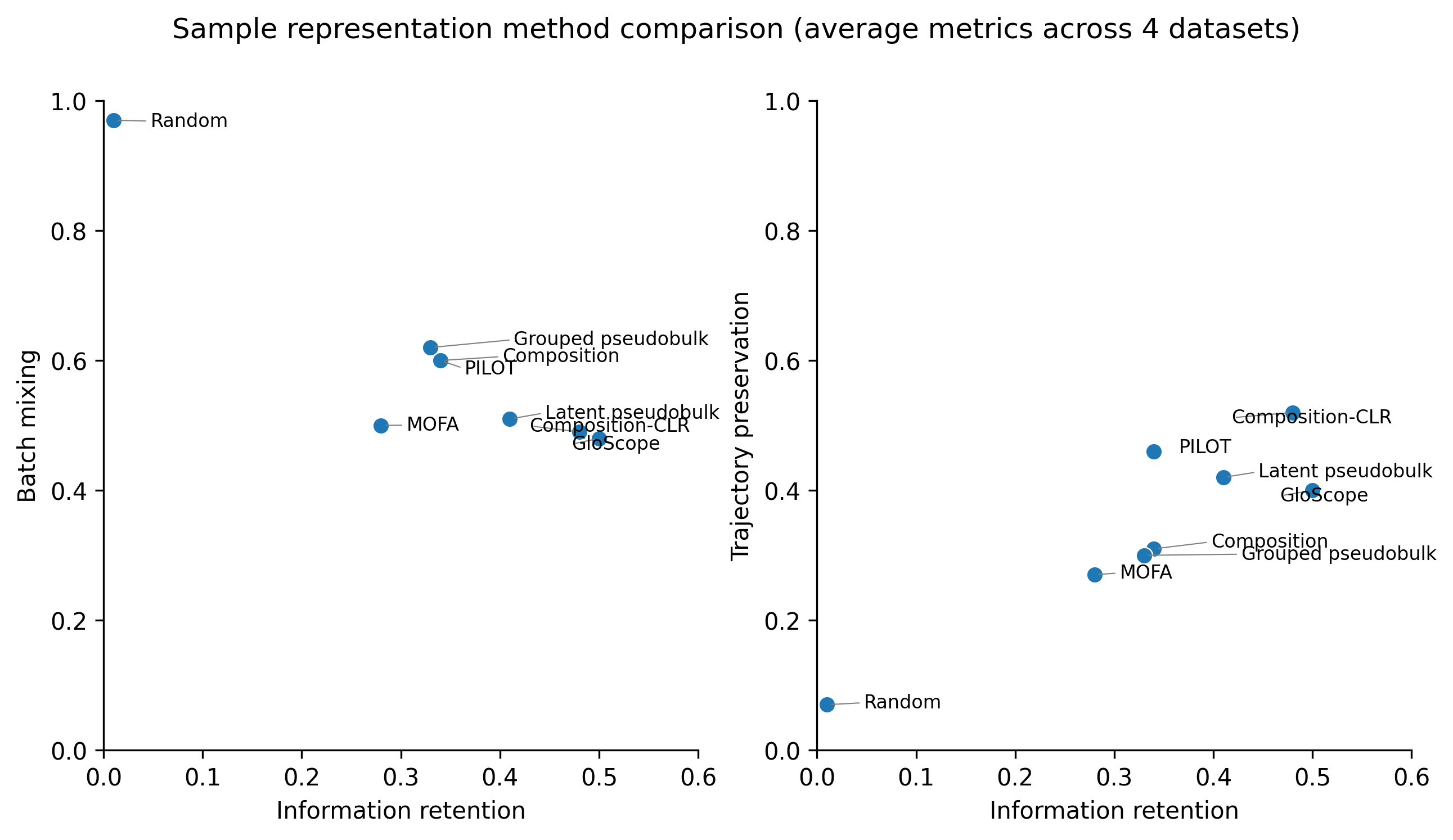
Reading the scatter: top-right = best on both criteria.

Note on coverage. Some methods are not run on every dataset, so their averaged scores aggregate over fewer datasets than others. GroupedPseudobulk is skipped on HLCA and OneK1K (the per-cell-type filter wipes too many sparse cell types at those donor counts). Every other method, including PILOT, runs on all four datasets. Read the per-method scores together with the runtime table below to see which methods contributed to each average.

Runtime per method per dataset (seconds)

runtime_table = pd.DataFrame(runtimes).round(1)
runtime_table["mean"] = runtime_table.mean(axis=1).round(1)
runtime_table.sort_values("mean")

	combat	hlca	stephenson	onek1k	mean
random_vec	0.0	0.0	0.0	0.1	0.0
composition_clr	0.2	0.7	0.2	0.4	0.4
grouped_pseudobulk	1.1	NaN	0.0	NaN	0.6
pseudobulk	0.3	1.8	0.3	1.9	1.1
composition	0.3	7.0	0.5	0.4	2.0
pilot	498.6	31.8	5.5	137.2	168.3
mofa	15.0	550.6	73.4	303.5	235.6
gloscope	246.9	205.6	32.8	892.7	344.5

We can see that baselines perform very strongly, especially CLR-transformed cell type composition. GloScope is the only method performing on par or better than the baselines for information retention, which we previously observed In the SPARE sample representation methods benchmark. PILOT on average performs well for trajectory preservation.

But as we have seen in this tutorial, performance of methods varies from one dataset to another. What works the best on average might hold for your data. Using patpy, you can quickly test what works for your case, and make the most from your data.

Other methods and tutorials

We covered Pseudobulk, GroupedPseudobulk, CellGroupComposition, PILOT, MOFA, GloScope (Python), and a RandomVector baseline. patpy also ships:

• patpy.tl.MrVI — deep generative model. Requires GPU and takes very long to run. It is more convenient to run it in a separate environment.

• patpy.tl.SCPoli — conditional VAE that learns a per-sample prototype, batch-aware by construction. Needs pip install patpy[scpoli] and (currently) an anndata < 0.12 env because scarches requirements.

• patpy.tl.DiffusionEarthMoverDistance — diffusion EMD over composition. Needs pip install patpy[diffusionemd] and scikit-learn < 1.5 for the underlying DiffusionEMD package.

Related tutorials:

• sources_of_variation_with_gloscope.ipynb — deep-dive on GloScope, including the R setup.

• supervised_methods_example.ipynb — running supervised methods fine-tuned for a specific covariate prediction (MixMIL, PULSAR, PaSCient) via patpy interface.

• differential_analysis.ipynb — interpreting sample-level variation with differential expression analysis.