Using supervised sample-level methods#
In this tutorial, we will demostrate how to run supervised sample-level methods for single-cell data with patpy.
Import packages#
import pandas as pd
import scanpy as sc
import patpy
import matplotlib.pyplot as plt
from sklearn.metrics import classification_report
patpy.__version__
'0.13.0'
Read the data#
Here, we use COMBAT dataset. This dataset contains 783k cells from 140 COVID-19 patients and healthy donors.
ADATA_PATH = "/home/icb/vladimir.shitov/projects/vladimir.shitov/2023_05_patient_representation_benchmark/reproducibility/pat_rep_benchmark/data/combat/combat_processed.h5ad"
adata = sc.read_h5ad(ADATA_PATH)
adata
AnnData object with n_obs × n_vars = 783677 × 3000
    obs: 'Annotation_cluster_id', 'Annotation_cluster_name', 'Annotation_minor_subset', 'Annotation_major_subset', 'Annotation_cell_type', 'GEX_region', 'QC_ngenes', 'QC_total_UMI', 'QC_pct_mitochondrial', 'QC_scrub_doublet_scores', 'TCR_chain_composition', 'TCR_clone_ID', 'TCR_clone_count', 'TCR_clone_proportion', 'TCR_contains_unproductive', 'TCR_doublet', 'TCR_chain_TRA', 'TCR_v_gene_TRA', 'TCR_d_gene_TRA', 'TCR_j_gene_TRA', 'TCR_c_gene_TRA', 'TCR_productive_TRA', 'TCR_cdr3_TRA', 'TCR_umis_TRA', 'TCR_chain_TRA2', 'TCR_v_gene_TRA2', 'TCR_d_gene_TRA2', 'TCR_j_gene_TRA2', 'TCR_c_gene_TRA2', 'TCR_productive_TRA2', 'TCR_cdr3_TRA2', 'TCR_umis_TRA2', 'TCR_chain_TRB', 'TCR_v_gene_TRB', 'TCR_d_gene_TRB', 'TCR_j_gene_TRB', 'TCR_c_gene_TRB', 'TCR_productive_TRB', 'TCR_chain_TRB2', 'TCR_v_gene_TRB2', 'TCR_d_gene_TRB2', 'TCR_j_gene_TRB2', 'TCR_c_gene_TRB2', 'TCR_productive_TRB2', 'TCR_cdr3_TRB2', 'TCR_umis_TRB2', 'BCR_umis_HC', 'BCR_contig_qc_HC', 'BCR_functionality_HC', 'BCR_v_call_HC', 'BCR_v_score_HC', 'BCR_j_call_HC', 'BCR_j_score_HC', 'BCR_junction_aa_HC', 'BCR_total_mut_HC', 'BCR_s_mut_HC', 'BCR_r_mut_HC', 'BCR_c_gene_HC', 'BCR_clone_per_replicate_HC', 'BCR_clone_global_HC', 'BCR_clonal_abundance_HC', 'BCR_locus_LC', 'BCR_umis_LC', 'BCR_contig_qc_LC', 'BCR_functionality_LC', 'BCR_v_call_LC', 'BCR_v_score_LC', 'BCR_j_call_LC', 'BCR_j_score_LC', 'BCR_junction_aa_LC', 'BCR_total_mut_LC', 'BCR_s_mut_LC', 'BCR_r_mut_LC', 'BCR_c_gene_LC', 'COMBAT_ID', 'scRNASeq_sample_ID', 'COMBAT_participant_timepoint_ID', 'Source', 'Age', 'Sex', 'Race', 'BMI', 'Hospitalstay', 'Death28', 'Institute', 'PreExistingHeartDisease', 'PreExistingLungDisease', 'PreExistingKidneyDisease', 'PreExistingDiabetes', 'PreExistingHypertension', 'PreExistingImmunocompromised', 'Smoking', 'Symptomatic', 'Requiredvasoactive', 'Respiratorysupport', 'SARSCoV2PCR', 'Outcome', 'TimeSinceOnset', 'Ethnicity', 'Tissue', 'DiseaseClassification', 'Pool_ID', 'Channel_ID', 'ifn_1_score', '_scvi_batch', '_scvi_labels', 'n_genes_by_counts', 'log1p_n_genes_by_counts', 'total_counts', 'log1p_total_counts', 'pct_counts_in_top_50_genes', 'pct_counts_in_top_100_genes', 'pct_counts_in_top_200_genes', 'pct_counts_in_top_500_genes', 'total_counts_mt', 'log1p_total_counts_mt', 'pct_counts_mt', 'total_counts_ribo', 'log1p_total_counts_ribo', 'pct_counts_ribo', 'vertex', 'eigenvector_centrality'
    var: 'gene_ids', 'feature_types', 'highly_variable', 'highly_variable_rank', 'means', 'variances', 'variances_norm', 'highly_variable_nbatches', 'mt', 'ribo', 'n_cells_by_counts', 'mean_counts', 'log1p_mean_counts', 'pct_dropout_by_counts', 'total_counts', 'log1p_total_counts'
    uns: 'Institute', 'ObjectCreateDate', 'Source_colors', 'Technology', 'X_gloscope_cuml_distances', 'X_gloscope_pynndescent_distances', 'X_scpoli', '_scvi_manager_uuid', '_scvi_uuid', 'genome_annotation_version', 'gloscope_representation', 'gloscope_scpoli_distances', 'hvg', 'log1p', 'neighbors', 'pca', 'scpoli_distances', 'scpoli_parameters', 'scpoli_samples'
    obsm: 'X_pca', 'X_scANVI_batch', 'X_scANVI_sample', 'X_scVI_batch', 'X_scVI_sample', 'X_scpoli', 'X_umap', 'X_umap_source'
    varm: 'PCs'
    layers: 'X_raw_counts'
    obsp: 'connectivities', 'distances'
Set columns containing sample IDs, cell types and metadata#
sample_id_col = "scRNASeq_sample_ID"
cell_type_key = "cell_type"
samples_metadata_cols = ["Source", "Outcome", "Death28", "Institute", "Pool_ID", "binary_condition"]
Currently, there is no such columns as “cell_type” in the data. But cell types are stored in the Annotation_major_subset column. Let’s rename it to cell_type for better readability.
adata.obs.rename(columns={"Annotation_major_subset": cell_type_key}, inplace=True)
For this tutorial, we will create a binaru condition column, containing information whether a donor is healthy or comes from COVID-19 group
adata = adata[~adata.obs["Source"].isin(["Sepsis", "Flu"])]
adata.obs["binary_condition"] = adata.obs["Source"].str.contains("COVID").astype(int) # 1 for COVID-19, 0 for healthy
adata.obs["binary_condition"].value_counts()
binary_condition
1    524530
0     87204
Name: count, dtype: int64
Store metadata and calculate QC metrics#
metadata = adata.obs[samples_metadata_cols + [sample_id_col]].drop_duplicates()
metadata.set_index(sample_id_col, inplace=True)
metadata
| Source | Outcome | Death28 | Institute | Pool_ID | binary_condition | |
|---|---|---|---|---|---|---|
| scRNASeq_sample_ID | ||||||
| S00109-Ja001E-PBCa | COVID_SEV | 2.0 | 0 | Oxford | gPlexA | 1 |
| S00112-Ja003E-PBCa | COVID_MILD | 5.0 | 0 | Oxford | gPlexA | 1 |
| S00005-Ja005E-PBCa | COVID_CRIT | 2.0 | 0 | Oxford | gPlexA | 1 |
| S00061-Ja003E-PBCa | COVID_SEV | 4.0 | 0 | Oxford | gPlexA | 1 |
| S00056-Ja003E-PBCa | COVID_SEV | 3.0 | 0 | Oxford | gPlexA | 1 |
| ... | ... | ... | ... | ... | ... | ... |
| S00076-Ja001E-PBCa | COVID_MILD | 5.0 | 0 | Oxford | gPlexK | 1 |
| S00072-Ja001E-PBCa | COVID_SEV | 2.0 | 0 | Oxford | gPlexK | 1 |
| S00065-Ja003E-PBCa | COVID_CRIT | 2.0 | 0 | Oxford | gPlexK | 1 |
| S00048-Ja003E-PBCa | COVID_SEV | 4.0 | 0 | Oxford | gPlexK | 1 |
| G05112-Ja005E-PBCa | COVID_HCW_MILD | 6.0 | 0 | Oxford | gPlexK | 1 |
101 rows × 6 columns
cell_qc_metadata = patpy.pp.calculate_cell_qc_metrics(
    adata, sample_key=sample_id_col, cell_qc_vars=["QC_ngenes", "QC_pct_mitochondrial", "QC_scrub_doublet_scores"]
)
n_cells_metadata = patpy.pp.calculate_n_cells_per_sample(adata, sample_id_col)
composition_metadata = patpy.pp.calculate_compositional_metrics(adata, sample_id_col, [cell_type_key], normalize_to=100)
metadata = pd.concat(
    [
        metadata,
        cell_qc_metadata.loc[metadata.index],
        n_cells_metadata.loc[metadata.index],
        composition_metadata.loc[metadata.index],
    ],
    axis=1,
)
metadata
| Source | Outcome | Death28 | Institute | Pool_ID | binary_condition | median_QC_ngenes | median_QC_pct_mitochondrial | median_QC_scrub_doublet_scores | n_cells | ... | cell_type_HSC | cell_type_MAIT | cell_type_Mast | cell_type_NK | cell_type_PB | cell_type_PLT | cell_type_RET | cell_type_cMono | cell_type_iNKT | cell_type_ncMono | |
|---|---|---|---|---|---|---|---|---|---|---|---|---|---|---|---|---|---|---|---|---|---|
| scRNASeq_sample_ID | |||||||||||||||||||||
| S00109-Ja001E-PBCa | COVID_SEV | 2.0 | 0 | Oxford | gPlexA | 1 | 1112.0 | 0.960763 | 0.036112 | 3984 | ... | 0.200803 | 1.004016 | 0.000000 | 20.682731 | 2.459839 | 0.075301 | 0.025100 | 28.664659 | 0.050201 | 1.079317 |
| S00112-Ja003E-PBCa | COVID_MILD | 5.0 | 0 | Oxford | gPlexA | 1 | 1068.0 | 1.286751 | 0.054808 | 7384 | ... | 0.135428 | 0.352113 | 0.000000 | 7.624594 | 2.816901 | 0.067714 | 0.000000 | 23.171723 | 0.013543 | 2.559588 |
| S00005-Ja005E-PBCa | COVID_CRIT | 2.0 | 0 | Oxford | gPlexA | 1 | 1123.0 | 1.176937 | 0.066325 | 9002 | ... | 0.099978 | 0.288825 | 0.000000 | 4.598978 | 1.832926 | 0.444346 | 0.000000 | 2.777161 | 0.000000 | 0.444346 |
| S00061-Ja003E-PBCa | COVID_SEV | 4.0 | 0 | Oxford | gPlexA | 1 | 1131.0 | 1.308555 | 0.044787 | 4278 | ... | 0.210379 | 0.327256 | 0.000000 | 8.952782 | 1.005143 | 0.116877 | 0.000000 | 43.010753 | 0.023375 | 3.295933 |
| S00056-Ja003E-PBCa | COVID_SEV | 3.0 | 0 | Oxford | gPlexA | 1 | 950.0 | 1.979107 | 0.053691 | 7600 | ... | 0.973684 | 0.039474 | 0.026316 | 5.263158 | 1.131579 | 0.236842 | 0.000000 | 39.960526 | 0.013158 | 2.486842 |
| ... | ... | ... | ... | ... | ... | ... | ... | ... | ... | ... | ... | ... | ... | ... | ... | ... | ... | ... | ... | ... | ... |
| S00076-Ja001E-PBCa | COVID_MILD | 5.0 | 0 | Oxford | gPlexK | 1 | 1251.0 | 2.055921 | 0.041096 | 5779 | ... | 0.069216 | 0.017304 | 0.017304 | 8.928880 | 0.242256 | 0.155736 | 0.000000 | 32.168195 | 0.017304 | 7.527254 |
| S00072-Ja001E-PBCa | COVID_SEV | 2.0 | 0 | Oxford | gPlexK | 1 | 1251.0 | 1.500790 | 0.037953 | 5195 | ... | 0.134745 | 0.538980 | 0.000000 | 12.281039 | 0.519731 | 0.076997 | 0.000000 | 19.037536 | 0.038499 | 1.828681 |
| S00065-Ja003E-PBCa | COVID_CRIT | 2.0 | 0 | Oxford | gPlexK | 1 | 1263.0 | 2.256898 | 0.049718 | 3924 | ... | 0.050968 | 0.050968 | 0.025484 | 3.211009 | 0.433231 | 0.127421 | 0.025484 | 38.863405 | 0.025484 | 4.306830 |
| S00048-Ja003E-PBCa | COVID_SEV | 4.0 | 0 | Oxford | gPlexK | 1 | 1140.0 | 2.032172 | 0.062704 | 3444 | ... | 0.290360 | 0.029036 | 0.000000 | 3.135889 | 1.596980 | 0.000000 | 0.000000 | 23.228804 | 0.058072 | 0.871080 |
| G05112-Ja005E-PBCa | COVID_HCW_MILD | 6.0 | 0 | Oxford | gPlexK | 1 | 1168.5 | 1.315744 | 0.042038 | 4432 | ... | 0.000000 | 0.135379 | 0.000000 | 3.249097 | 0.473827 | 0.000000 | 0.000000 | 27.098375 | 0.000000 | 5.956679 |
101 rows × 27 columns
Quality control#
To reduce noise in the representations, we need to remove samples with too few cells:
adata = patpy.pp.filter_small_samples(adata, sample_key=sample_id_col, sample_size_threshold=250)
0 samples removed:
Run MixMIL#
MixMIL is a method, combining mixed models and multiple instance learning. It learns importance of each cell for a supervised task, aggregates cells with these learned weights, and predicts a label of interest. MixedMIL is a light-weight model and is a great baseline for supervised sample-level tasks. Here, we will show how to use it via patpy to distinguish healthy people from COVID-19 patients
Initialize MixMIL. Select the layer you would like to use and a list of tasks. Supported tasks are:
"classification""regression"
mixmil = patpy.tl.supervised.MixMIL(
    sample_key=sample_id_col,
    label_keys=["binary_condition"],
    tasks=["classification"],
    layer="X_pca",
    n_epochs=100
)
Train the MixMIL model:
mixmil.prepare_anndata(adata)
We can now display the training history:
losses = [step["loss"] for step in mixmil.training_history]
plt.plot(losses, label="MixMIL loss")
plt.xlabel("Optimiser step")
plt.ylabel("Loss")
Text(0, 0.5, 'Loss')
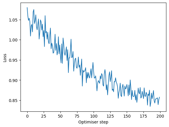
The loss is going down, which is a desired behavior. Note that the number of steps here is bigger than the number of epochs we set. This is because training history contains information for every minibatch of the data. For this dataset and batch size, every epoch consists of 2 steps.
We can now obtain sample embeddings from the model:
mixmil_sample_reps = mixmil.get_sample_representations()
mixmil_sample_reps
| dim_0 | dim_1 | dim_2 | dim_3 | dim_4 | dim_5 | dim_6 | dim_7 | dim_8 | dim_9 | ... | dim_40 | dim_41 | dim_42 | dim_43 | dim_44 | dim_45 | dim_46 | dim_47 | dim_48 | dim_49 | |
|---|---|---|---|---|---|---|---|---|---|---|---|---|---|---|---|---|---|---|---|---|---|
| G05061-Ja005E-PBCa | -1.381277 | 1.341956 | -0.457196 | -1.456421 | -0.330128 | -1.155065 | -0.913108 | 0.521566 | 0.298353 | 0.858071 | ... | 0.050455 | 0.191479 | -0.086966 | -0.146908 | 0.049881 | 0.067801 | 0.042632 | -0.081675 | -0.021801 | -0.128855 |
| G05064-Ja005E-PBCa | -0.840356 | -0.758498 | -0.385595 | -0.936781 | -1.270981 | -0.677239 | -0.238136 | -0.872834 | 0.775794 | 0.139842 | ... | -0.000316 | 0.086494 | -0.003116 | -0.167811 | 0.169646 | -0.017056 | 0.009289 | -0.028307 | -0.022568 | 0.024029 |
| G05073-Ja005E-PBCa | -0.538473 | 0.331862 | -0.132182 | -0.686238 | -0.267157 | -1.316424 | 0.237110 | 0.957211 | 0.683576 | 0.903618 | ... | 0.118959 | 0.088980 | -0.039237 | 0.130772 | 0.141599 | 0.017822 | 0.017913 | 0.070581 | 0.083621 | -0.170728 |
| G05077-Ja005E-PBCa | -0.527064 | 1.900464 | 0.300888 | -1.442165 | -0.584309 | -1.436059 | -0.178377 | 0.058934 | 0.615683 | 0.767669 | ... | 0.176571 | 0.101752 | -0.059887 | 0.181135 | 0.034280 | -0.056092 | 0.019616 | -0.028876 | 0.061174 | -0.013765 |
| G05078-Ja005E-PBCa | -0.832603 | -0.414575 | -0.206571 | -1.346403 | -0.957619 | -1.585800 | -0.586254 | -0.052773 | 0.419745 | 0.945472 | ... | 0.443253 | 0.189156 | -0.111214 | 0.076169 | 0.133255 | -0.042016 | 0.110961 | -0.142148 | 0.008514 | -0.070022 |
| ... | ... | ... | ... | ... | ... | ... | ... | ... | ... | ... | ... | ... | ... | ... | ... | ... | ... | ... | ... | ... | ... |
| S00134-Ja003E-PBCa | 6.941552 | 0.031779 | -0.624828 | -0.280828 | 0.296835 | -0.387412 | -0.449077 | 0.100738 | -0.125929 | 0.074249 | ... | -0.038420 | 0.005695 | -0.039585 | 0.186113 | -0.074605 | 0.083164 | -0.013090 | 0.004723 | 0.080961 | 0.004850 |
| S00142-Ja005E-PBCa | 3.097914 | 2.850465 | 1.051137 | 0.121225 | 0.224610 | -0.820552 | -0.150583 | 0.094237 | 0.402730 | 0.786933 | ... | -0.136479 | 0.091933 | 0.033427 | 0.008240 | 0.021939 | 0.000124 | 0.152159 | -0.048620 | -0.033645 | 0.021786 |
| S00148-Ja003E-PBCa | 0.750430 | 2.372979 | 0.146777 | 0.036760 | -0.081484 | -0.807887 | 0.507421 | 0.357030 | 0.096658 | -0.360064 | ... | -0.073529 | -0.368383 | -0.052634 | 0.215808 | -0.031842 | 0.076604 | 0.132863 | 0.085280 | -0.031466 | 0.029088 |
| U00515-Ua005E-PBUa | -1.533610 | 0.573506 | -0.563373 | 0.437439 | -0.800104 | -0.947790 | 0.095739 | -0.886351 | 0.364036 | -0.315162 | ... | -0.231965 | -0.142485 | -0.208615 | -0.331639 | -0.022948 | -0.172401 | 0.108861 | 0.008939 | 0.078424 | 0.112581 |
| U00519-Ua005E-PBUa | -2.315831 | 1.010524 | -0.536370 | 0.538096 | -0.152678 | -0.441404 | -0.159282 | -0.569883 | -0.522771 | 0.313985 | ... | 0.136863 | 0.156610 | 0.081693 | 0.005688 | -0.115762 | -0.022072 | 0.062207 | 0.040832 | 0.066958 | 0.014584 |
101 rows × 50 columns
And apply our evaluation metrics to them. Here, we test how well binary condition is predicted from the nearest neighbors in the sample representation space:
mixmil_distances = mixmil.calculate_distance_matrix()
patpy.tl.evaluate_representation(
    mixmil_distances,
    target=metadata.loc[mixmil.samples, "binary_condition"],
    task="classification"
)
{'score': np.float64(0.5933275812482024),
 'metric': 'f1_macro_calibrated',
 'n_unique': 2,
 'n_observations': 101,
 'method': 'knn'}
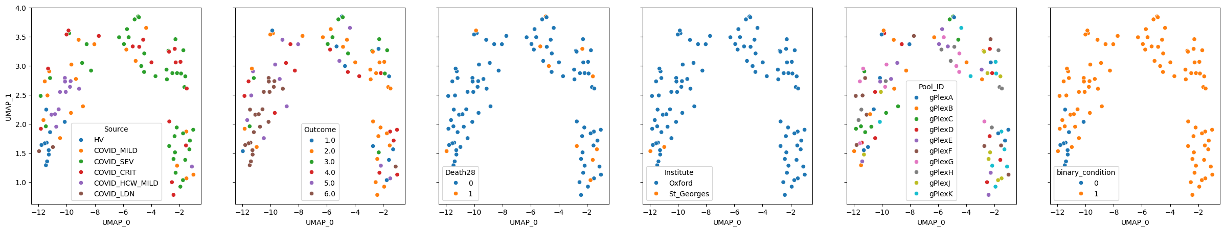
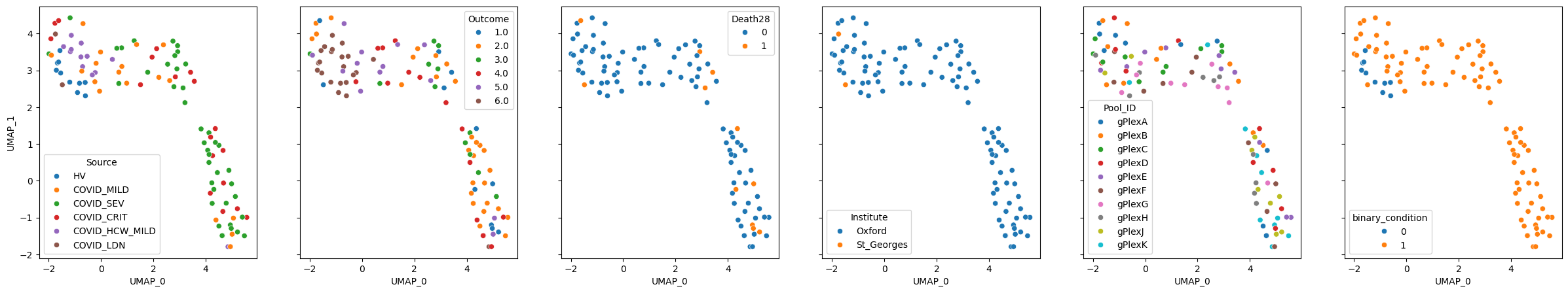
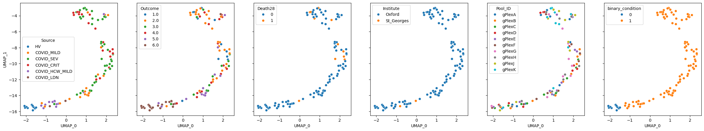
We can then visualise sample representation using dimensionality reduction methods:
mixmil.plot_embedding(method="UMAP", metadata_cols=samples_metadata_cols, continuous_palette="tab10");
Additionally, we can predict a label directly with the model:
mixmil_prediction = mixmil.predict("binary_condition")
mixmil_prediction
| prob_0 | prob_1 | binary_condition_pred | |
|---|---|---|---|
| G05061-Ja005E-PBCa | 0.536446 | 0.463554 | 0 |
| G05064-Ja005E-PBCa | 0.524378 | 0.475622 | 0 |
| G05073-Ja005E-PBCa | 0.522635 | 0.477365 | 0 |
| G05077-Ja005E-PBCa | 0.533199 | 0.466801 | 0 |
| G05078-Ja005E-PBCa | 0.537712 | 0.462288 | 0 |
| ... | ... | ... | ... |
| S00134-Ja003E-PBCa | 0.489505 | 0.510495 | 1 |
| S00142-Ja005E-PBCa | 0.509378 | 0.490622 | 0 |
| S00148-Ja003E-PBCa | 0.520626 | 0.479374 | 0 |
| U00515-Ua005E-PBUa | 0.533269 | 0.466731 | 0 |
| U00519-Ua005E-PBUa | 0.551527 | 0.448473 | 0 |
101 rows × 3 columns
# Make sure that the order of labels is the same in metadata and prediction
y_true = metadata.loc[mixmil_prediction.index, "binary_condition"]
print(classification_report(y_true, mixmil_prediction["binary_condition_pred"]))
              precision    recall  f1-score   support

           0       0.19      1.00      0.32        10
           1       1.00      0.53      0.69        91

    accuracy                           0.57       101
   macro avg       0.59      0.76      0.50       101
weighted avg       0.92      0.57      0.65       101
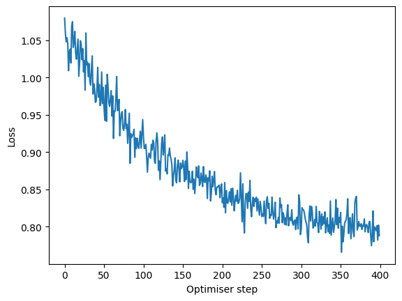
The prediction is not perfect, but the model is not fully trained as you can see on the loss plot. Let’s train it a bit further with a fine_tune method:
mixmil.fine_tune("binary_condition", tasks="classification", n_epochs=100, lr=0.001)
losses = [step["loss"] for step in mixmil.training_history]
plt.plot(losses, label="MixMIL loss")
plt.xlabel("Optimiser step")
plt.ylabel("Loss")
Text(0, 0.5, 'Loss')
mixmil_prediction = mixmil.predict("binary_condition")

y_true = metadata.loc[mixmil_prediction.index, "binary_condition"]
print(classification_report(y_true, mixmil_prediction["binary_condition_pred"]))
              precision    recall  f1-score   support

           0       0.19      1.00      0.32        10
           1       1.00      0.53      0.69        91

    accuracy                           0.57       101
   macro avg       0.59      0.76      0.50       101
weighted avg       0.92      0.57      0.65       101
Interestingly, fine-tuning did not increase the metrics.
Additionally, the model can be fine-tuned for other tasks. For example, let’s add classification of all the disease labels:
metadata["Source"].value_counts()
Source
COVID_SEV         41
COVID_MILD        18
COVID_CRIT        18
COVID_HCW_MILD    12
HV                10
COVID_LDN          2
Name: count, dtype: int64
mixmil.fine_tune("Source", tasks="classification", n_epochs=100, lr=0.001)
losses = [step["loss"] for step in mixmil.training_history]
plt.plot(losses, label="MixMIL loss")
plt.xlabel("Optimiser step")
plt.ylabel("Loss")
Text(0, 0.5, 'Loss')
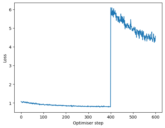
The loss initially jumped, but this is expected because the multi-label classification task is more challenging.
We can now predict the source labels:
mixmil_source_prediction = mixmil.predict("Source")
mixmil_source_prediction
| prob_COVID_CRIT | prob_COVID_HCW_MILD | prob_COVID_LDN | prob_COVID_MILD | prob_COVID_SEV | prob_HV | Source_pred | |
|---|---|---|---|---|---|---|---|
| G05061-Ja005E-PBCa | 0.030640 | 0.561769 | 0.074374 | 0.072961 | 0.032138 | 0.228119 | COVID_HCW_MILD |
| G05064-Ja005E-PBCa | 0.029576 | 0.642543 | 0.096133 | 0.066386 | 0.032763 | 0.132599 | COVID_HCW_MILD |
| G05073-Ja005E-PBCa | 0.029037 | 0.696279 | 0.060170 | 0.065821 | 0.030582 | 0.118111 | COVID_HCW_MILD |
| G05077-Ja005E-PBCa | 0.033331 | 0.591017 | 0.072786 | 0.068909 | 0.032433 | 0.201525 | COVID_HCW_MILD |
| G05078-Ja005E-PBCa | 0.027393 | 0.656529 | 0.072747 | 0.048350 | 0.023097 | 0.171884 | COVID_HCW_MILD |
| ... | ... | ... | ... | ... | ... | ... | ... |
| S00134-Ja003E-PBCa | 0.231576 | 0.125973 | 0.127787 | 0.131656 | 0.239131 | 0.143877 | COVID_SEV |
| S00142-Ja005E-PBCa | 0.102261 | 0.205523 | 0.118141 | 0.170917 | 0.131285 | 0.271872 | HV |
| S00148-Ja003E-PBCa | 0.089273 | 0.206138 | 0.137493 | 0.149648 | 0.101961 | 0.315488 | HV |
| U00515-Ua005E-PBUa | 0.094870 | 0.181981 | 0.220683 | 0.098946 | 0.057235 | 0.346284 | HV |
| U00519-Ua005E-PBUa | 0.113143 | 0.043682 | 0.257834 | 0.075100 | 0.059250 | 0.450991 | HV |
101 rows × 7 columns
source_true = metadata.loc[mixmil_source_prediction.index, "Source"]
print(classification_report(source_true, mixmil_source_prediction["Source_pred"]))
                precision    recall  f1-score   support

    COVID_CRIT       0.55      0.67      0.60        18
COVID_HCW_MILD       0.44      1.00      0.62        12
     COVID_LDN       0.00      0.00      0.00         2
    COVID_MILD       0.00      0.00      0.00        18
     COVID_SEV       0.83      0.46      0.59        41
            HV       0.37      1.00      0.54        10

      accuracy                           0.52       101
     macro avg       0.36      0.52      0.39       101
  weighted avg       0.52      0.52      0.47       101
The model is now trained to jointly predict binary condition and source:
mixmil.label_keys
['binary_condition', 'Source']
We can therefore predict both labels:
mixmil_binary_prediction = mixmil.predict("binary_condition")
binary_condition_true = metadata.loc[mixmil_binary_prediction.index, "binary_condition"]
print(classification_report(y_true, mixmil_binary_prediction["binary_condition_pred"]))
              precision    recall  f1-score   support

           0       0.19      1.00      0.32        10
           1       1.00      0.53      0.69        91

    accuracy                           0.57       101
   macro avg       0.59      0.76      0.50       101
weighted avg       0.92      0.57      0.65       101
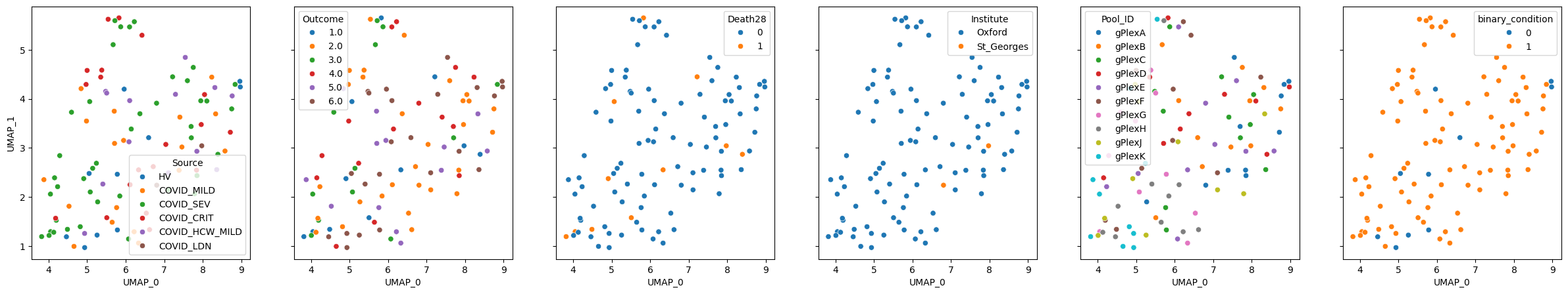
Let’s see how the model represents samples now. We must recompute distances matrix and update the UMAP, otherwise an old embedding will be used:
mixmil.calculate_distance_matrix()
mixmil.embed("UMAP")
mixmil.plot_embedding(method="UMAP", metadata_cols=samples_metadata_cols, continuous_palette="tab10");
Running PULSAR#
Install helical to get UCE embeddings. You can use envs/helical.yaml conda file in the patpy source directory for an easier installation.
!pip install patpy[helical]
We need to load the data with raw counts to obtain UCE embeddings
adata = sc.read_h5ad("/home/icb/vladimir.shitov/projects/vladimir.shitov/2023_05_patient_representation_benchmark/reproducibility/pat_rep_benchmark/data/combat/combat.h5ad")
adata
AnnData object with n_obs × n_vars = 836148 × 20807
    obs: 'Annotation_cluster_id', 'Annotation_cluster_name', 'Annotation_minor_subset', 'Annotation_major_subset', 'Annotation_cell_type', 'GEX_region', 'QC_ngenes', 'QC_total_UMI', 'QC_pct_mitochondrial', 'QC_scrub_doublet_scores', 'TCR_chain_composition', 'TCR_clone_ID', 'TCR_clone_count', 'TCR_clone_proportion', 'TCR_contains_unproductive', 'TCR_doublet', 'TCR_chain_TRA', 'TCR_v_gene_TRA', 'TCR_d_gene_TRA', 'TCR_j_gene_TRA', 'TCR_c_gene_TRA', 'TCR_productive_TRA', 'TCR_cdr3_TRA', 'TCR_umis_TRA', 'TCR_chain_TRA2', 'TCR_v_gene_TRA2', 'TCR_d_gene_TRA2', 'TCR_j_gene_TRA2', 'TCR_c_gene_TRA2', 'TCR_productive_TRA2', 'TCR_cdr3_TRA2', 'TCR_umis_TRA2', 'TCR_chain_TRB', 'TCR_v_gene_TRB', 'TCR_d_gene_TRB', 'TCR_j_gene_TRB', 'TCR_c_gene_TRB', 'TCR_productive_TRB', 'TCR_chain_TRB2', 'TCR_v_gene_TRB2', 'TCR_d_gene_TRB2', 'TCR_j_gene_TRB2', 'TCR_c_gene_TRB2', 'TCR_productive_TRB2', 'TCR_cdr3_TRB2', 'TCR_umis_TRB2', 'BCR_umis_HC', 'BCR_contig_qc_HC', 'BCR_functionality_HC', 'BCR_v_call_HC', 'BCR_v_score_HC', 'BCR_j_call_HC', 'BCR_j_score_HC', 'BCR_junction_aa_HC', 'BCR_total_mut_HC', 'BCR_s_mut_HC', 'BCR_r_mut_HC', 'BCR_c_gene_HC', 'BCR_clone_per_replicate_HC', 'BCR_clone_global_HC', 'BCR_clonal_abundance_HC', 'BCR_locus_LC', 'BCR_umis_LC', 'BCR_contig_qc_LC', 'BCR_functionality_LC', 'BCR_v_call_LC', 'BCR_v_score_LC', 'BCR_j_call_LC', 'BCR_j_score_LC', 'BCR_junction_aa_LC', 'BCR_total_mut_LC', 'BCR_s_mut_LC', 'BCR_r_mut_LC', 'BCR_c_gene_LC', 'COMBAT_ID', 'scRNASeq_sample_ID', 'COMBAT_participant_timepoint_ID', 'Source', 'Age', 'Sex', 'Race', 'BMI', 'Hospitalstay', 'Death28', 'Institute', 'PreExistingHeartDisease', 'PreExistingLungDisease', 'PreExistingKidneyDisease', 'PreExistingDiabetes', 'PreExistingHypertension', 'PreExistingImmunocompromised', 'Smoking', 'Symptomatic', 'Requiredvasoactive', 'Respiratorysupport', 'SARSCoV2PCR', 'Outcome', 'TimeSinceOnset', 'Ethnicity', 'Tissue', 'DiseaseClassification', 'Pool_ID', 'Channel_ID'
    var: 'gene_ids', 'feature_types'
    uns: 'Institute', 'ObjectCreateDate', 'Source_colors', 'Technology', 'genome_annotation_version'
    obsm: 'X_umap', 'X_umap_source'
    layers: 'raw'
adata.layers["raw"][:30, :30].A
array([[0., 0., 0., 0., 1., 0., 0., 0., 0., 0., 0., 0., 0., 0., 0., 0.,
        0., 0., 0., 0., 0., 0., 0., 0., 0., 0., 0., 0., 2., 0.],
       [0., 0., 0., 0., 0., 0., 0., 0., 0., 1., 0., 0., 0., 0., 0., 0.,
        0., 0., 0., 0., 0., 0., 0., 0., 0., 0., 0., 0., 0., 0.],
       [0., 0., 0., 0., 0., 0., 0., 0., 0., 0., 0., 0., 0., 0., 0., 0.,
        0., 0., 0., 0., 0., 0., 0., 0., 0., 0., 0., 0., 1., 1.],
       [0., 0., 0., 0., 1., 0., 0., 0., 0., 2., 0., 0., 0., 0., 0., 0.,
        0., 0., 0., 0., 0., 0., 1., 1., 0., 0., 0., 0., 0., 0.],
       [0., 0., 0., 0., 1., 0., 0., 0., 0., 8., 1., 0., 0., 0., 0., 0.,
        0., 0., 0., 0., 0., 0., 0., 0., 0., 0., 0., 0., 1., 0.],
       [0., 0., 0., 0., 0., 0., 0., 0., 0., 0., 0., 0., 0., 0., 0., 0.,
        1., 0., 0., 0., 0., 1., 0., 0., 0., 0., 0., 0., 0., 0.],
       [0., 0., 0., 0., 0., 0., 0., 0., 0., 0., 0., 0., 0., 0., 0., 0.,
        0., 0., 0., 0., 0., 0., 0., 0., 0., 0., 0., 0., 0., 0.],
       [0., 0., 0., 0., 1., 0., 0., 0., 0., 0., 0., 0., 0., 0., 0., 0.,
        0., 0., 0., 0., 0., 0., 0., 1., 0., 0., 0., 0., 1., 0.],
       [0., 0., 0., 0., 0., 0., 0., 0., 0., 0., 0., 0., 0., 0., 0., 0.,
        0., 0., 0., 0., 0., 0., 0., 0., 0., 0., 0., 0., 1., 0.],
       [0., 0., 0., 0., 0., 0., 0., 0., 0., 0., 0., 0., 0., 0., 0., 0.,
        0., 0., 0., 0., 0., 0., 0., 0., 0., 0., 0., 0., 0., 0.],
       [0., 0., 0., 0., 0., 0., 0., 0., 0., 0., 0., 0., 0., 0., 0., 0.,
        0., 0., 0., 0., 0., 0., 0., 0., 0., 0., 0., 0., 2., 0.],
       [0., 0., 0., 0., 0., 0., 0., 0., 0., 1., 0., 0., 0., 0., 0., 0.,
        1., 0., 0., 0., 0., 0., 0., 0., 0., 0., 0., 0., 0., 1.],
       [0., 0., 0., 0., 1., 0., 0., 0., 0., 1., 0., 0., 0., 0., 0., 0.,
        0., 0., 0., 0., 0., 0., 0., 0., 0., 0., 0., 0., 0., 0.],
       [0., 0., 0., 0., 0., 0., 0., 0., 0., 0., 0., 0., 0., 0., 1., 0.,
        1., 0., 0., 0., 0., 0., 0., 0., 0., 0., 0., 0., 1., 0.],
       [0., 0., 0., 0., 0., 0., 0., 0., 0., 0., 0., 0., 0., 0., 0., 0.,
        1., 0., 0., 1., 0., 0., 0., 0., 0., 0., 0., 0., 2., 0.],
       [0., 0., 0., 0., 0., 0., 0., 0., 0., 2., 0., 0., 0., 0., 0., 0.,
        0., 0., 0., 0., 0., 0., 0., 0., 0., 0., 0., 0., 0., 0.],
       [0., 0., 0., 0., 0., 0., 0., 0., 0., 0., 0., 0., 0., 0., 0., 0.,
        0., 0., 0., 0., 0., 0., 0., 0., 0., 0., 0., 0., 0., 0.],
       [0., 0., 0., 0., 1., 0., 0., 0., 0., 0., 0., 0., 0., 0., 0., 0.,
        0., 0., 0., 0., 0., 0., 0., 1., 0., 0., 0., 0., 1., 0.],
       [0., 0., 0., 0., 0., 0., 0., 0., 0., 0., 0., 0., 0., 0., 0., 0.,
        0., 0., 0., 0., 0., 0., 0., 1., 0., 0., 0., 0., 1., 0.],
       [0., 0., 0., 0., 0., 0., 0., 0., 0., 0., 0., 0., 0., 0., 0., 0.,
        1., 0., 0., 2., 0., 0., 0., 1., 0., 1., 0., 0., 0., 0.],
       [0., 0., 0., 0., 0., 0., 0., 0., 0., 0., 0., 0., 0., 0., 0., 0.,
        0., 0., 0., 0., 0., 0., 0., 0., 0., 0., 0., 0., 0., 0.],
       [0., 0., 0., 0., 0., 0., 0., 0., 0., 0., 0., 0., 0., 0., 0., 0.,
        0., 0., 0., 0., 0., 0., 0., 0., 0., 0., 0., 0., 0., 1.],
       [0., 0., 0., 0., 1., 0., 0., 0., 0., 0., 0., 0., 0., 0., 0., 0.,
        0., 0., 0., 0., 0., 0., 0., 0., 0., 0., 0., 0., 1., 0.],
       [0., 0., 0., 0., 0., 0., 0., 0., 0., 0., 0., 0., 0., 0., 0., 0.,
        1., 0., 0., 0., 0., 0., 0., 1., 0., 0., 0., 0., 0., 0.],
       [0., 0., 0., 0., 0., 0., 0., 0., 0., 2., 0., 0., 0., 0., 0., 0.,
        0., 0., 0., 0., 0., 0., 0., 1., 0., 0., 0., 0., 1., 0.],
       [0., 0., 0., 0., 0., 0., 0., 0., 0., 1., 0., 0., 0., 0., 0., 0.,
        0., 0., 0., 0., 0., 0., 0., 0., 0., 0., 0., 0., 0., 0.],
       [0., 0., 0., 0., 1., 0., 0., 0., 0., 0., 0., 0., 0., 0., 0., 0.,
        0., 0., 0., 1., 0., 0., 0., 0., 0., 0., 0., 0., 1., 0.],
       [0., 0., 0., 0., 0., 0., 0., 0., 0., 0., 0., 0., 0., 0., 0., 0.,
        1., 0., 0., 1., 0., 0., 0., 0., 0., 0., 0., 0., 0., 0.],
       [0., 0., 0., 0., 0., 0., 0., 0., 0., 4., 0., 0., 0., 0., 0., 0.,
        0., 0., 0., 0., 0., 0., 0., 0., 0., 0., 0., 0., 0., 0.],
       [0., 0., 0., 0., 0., 0., 0., 0., 0., 1., 0., 0., 0., 0., 2., 3.,
        0., 0., 0., 0., 0., 0., 0., 1., 0., 0., 0., 0., 1., 1.]],
      dtype=float32)
adata.X = adata.layers["raw"]
Let’s subsample our data object to 1024 cells per sample that PULSAR uses. This will also drastically reduce time to get UCE embeddings
adata = patpy.pp.subsample(adata, obs_category_col=sample_id_col, n_obs=1024, min_samples_per_category=250)
adata
View of AnnData object with n_obs × n_vars = 103460 × 20807
    obs: 'Annotation_cluster_id', 'Annotation_cluster_name', 'Annotation_minor_subset', 'cell_type', 'Annotation_cell_type', 'GEX_region', 'QC_ngenes', 'QC_total_UMI', 'QC_pct_mitochondrial', 'QC_scrub_doublet_scores', 'TCR_chain_composition', 'TCR_clone_ID', 'TCR_clone_count', 'TCR_clone_proportion', 'TCR_contains_unproductive', 'TCR_doublet', 'TCR_chain_TRA', 'TCR_v_gene_TRA', 'TCR_d_gene_TRA', 'TCR_j_gene_TRA', 'TCR_c_gene_TRA', 'TCR_productive_TRA', 'TCR_cdr3_TRA', 'TCR_umis_TRA', 'TCR_chain_TRA2', 'TCR_v_gene_TRA2', 'TCR_d_gene_TRA2', 'TCR_j_gene_TRA2', 'TCR_c_gene_TRA2', 'TCR_productive_TRA2', 'TCR_cdr3_TRA2', 'TCR_umis_TRA2', 'TCR_chain_TRB', 'TCR_v_gene_TRB', 'TCR_d_gene_TRB', 'TCR_j_gene_TRB', 'TCR_c_gene_TRB', 'TCR_productive_TRB', 'TCR_chain_TRB2', 'TCR_v_gene_TRB2', 'TCR_d_gene_TRB2', 'TCR_j_gene_TRB2', 'TCR_c_gene_TRB2', 'TCR_productive_TRB2', 'TCR_cdr3_TRB2', 'TCR_umis_TRB2', 'BCR_umis_HC', 'BCR_contig_qc_HC', 'BCR_functionality_HC', 'BCR_v_call_HC', 'BCR_v_score_HC', 'BCR_j_call_HC', 'BCR_j_score_HC', 'BCR_junction_aa_HC', 'BCR_total_mut_HC', 'BCR_s_mut_HC', 'BCR_r_mut_HC', 'BCR_c_gene_HC', 'BCR_clone_per_replicate_HC', 'BCR_clone_global_HC', 'BCR_clonal_abundance_HC', 'BCR_locus_LC', 'BCR_umis_LC', 'BCR_contig_qc_LC', 'BCR_functionality_LC', 'BCR_v_call_LC', 'BCR_v_score_LC', 'BCR_j_call_LC', 'BCR_j_score_LC', 'BCR_junction_aa_LC', 'BCR_total_mut_LC', 'BCR_s_mut_LC', 'BCR_r_mut_LC', 'BCR_c_gene_LC', 'COMBAT_ID', 'scRNASeq_sample_ID', 'COMBAT_participant_timepoint_ID', 'Source', 'Age', 'Sex', 'Race', 'BMI', 'Hospitalstay', 'Death28', 'Institute', 'PreExistingHeartDisease', 'PreExistingLungDisease', 'PreExistingKidneyDisease', 'PreExistingDiabetes', 'PreExistingHypertension', 'PreExistingImmunocompromised', 'Smoking', 'Symptomatic', 'Requiredvasoactive', 'Respiratorysupport', 'SARSCoV2PCR', 'Outcome', 'TimeSinceOnset', 'Ethnicity', 'Tissue', 'DiseaseClassification', 'Pool_ID', 'Channel_ID', 'binary_condition'
    var: 'gene_ids', 'feature_types'
    uns: 'Institute', 'ObjectCreateDate', 'Source_colors', 'Technology', 'genome_annotation_version'
    obsm: 'X_umap', 'X_umap_source'
    layers: 'raw'
adata = patpy.pp.basic.get_helical_embedding(adata, model="uce", device="cuda")
adata.obsm["X_uce"].shape
(103460, 1280)
Now goes a bit annoying part… At teh time of writing this tutorial, helical requires python version <3.13. And to run PULSAR, we need python >= 3.13. So we need to save the object with UCE embeddings now, change the environment to the one containin python 3.13 and run PULSAR from there.
adata.write_h5ad("data/combat_subsample_with_uce.h5ad")
Load the data after switching the environment
adata = sc.read_h5ad("data/combat_subsample_with_uce.h5ad")
adata.obsm["X_uce"].shape
(103460, 1280)
You can now run PULSAR via patpy. Before doing that, make sure to install it by running pip install git+https://github.com/snap-stanford/PULSAR
pulsar = patpy.tl.supervised.PULSAR(
    sample_key=sample_id_col,
    label_keys=["binary_condition"],
    tasks=["classification"]
)
pulsar.prepare_anndata(adata)
Resample 0 time
pulsar_distances = pulsar.calculate_distance_matrix()
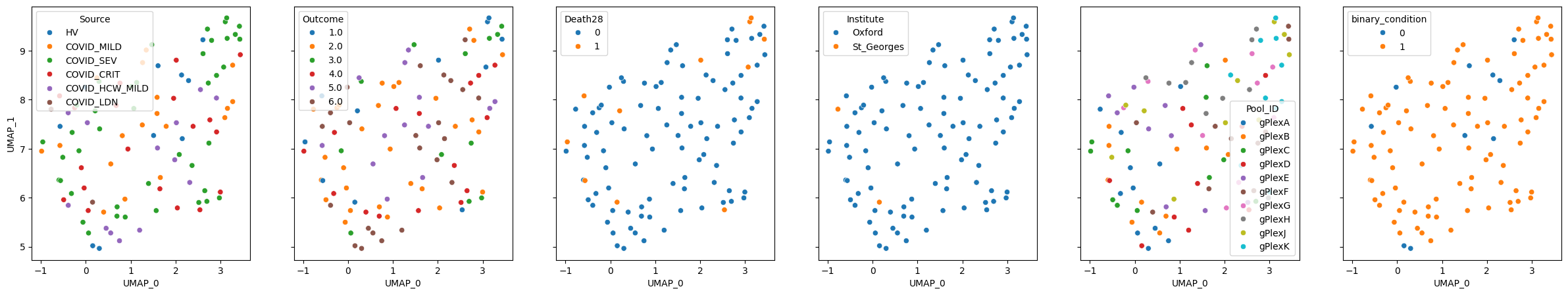
pulsar.plot_embedding(method="UMAP", metadata_cols=samples_metadata_cols, continuous_palette="tab10");
As we can see, the model doesn’t preserve information particularly well, despite being trained on this dataset and having 87 million parameters (on top of underlying 650M for UCE and 15B for ESM2)
Let’s give PULSAR another change and load the model fine-tuned for disease prediction
pulsar_aligned = patpy.tl.supervised.PULSAR(
    sample_key=sample_id_col,
    label_keys=["binary_condition"],
    tasks=["classification"],
    pretrained_model="KuanP/PULSAR-aligned"
)
pulsar_aligned.prepare_anndata(adata)
Resample 0 time
pulsar_aligned_distances = pulsar_aligned.calculate_distance_matrix()
pulsar_aligned.plot_embedding(method="UMAP", metadata_cols=samples_metadata_cols, continuous_palette="tab10");
We can run apply fine_tune to PULSAR as well. In this case, the base model won’t be retrained, but instead a small linear classifier will be trained on top of it. We can add as many prediction tasks as we want, they will be trained independently from each other.
pulsar.fine_tune(
    labels=["binary_condition", "Source"],
    tasks=["classification", "classification"]
)
pulsar_source_prediction = pulsar.predict("Source")
pulsar_source_prediction
| prob_COVID_CRIT | prob_COVID_HCW_MILD | prob_COVID_LDN | prob_COVID_MILD | prob_COVID_SEV | prob_HV | Source_pred | |
|---|---|---|---|---|---|---|---|
| S00109-Ja001E-PBCa | 0.179383 | 0.138693 | 0.154339 | 0.159889 | 0.199176 | 0.168521 | COVID_SEV |
| S00112-Ja003E-PBCa | 0.145783 | 0.164913 | 0.168011 | 0.202601 | 0.146124 | 0.172568 | COVID_MILD |
| G05153-Ja005E-PBCa | 0.145258 | 0.215347 | 0.194767 | 0.139690 | 0.137902 | 0.167036 | COVID_HCW_MILD |
| S00005-Ja005E-PBCa | 0.162052 | 0.169440 | 0.203298 | 0.152381 | 0.157898 | 0.154931 | COVID_LDN |
| S00061-Ja003E-PBCa | 0.165861 | 0.158230 | 0.187931 | 0.165523 | 0.166231 | 0.156225 | COVID_LDN |
| ... | ... | ... | ... | ... | ... | ... | ... |
| S00076-Ja001E-PBCa | 0.176172 | 0.156331 | 0.098420 | 0.195909 | 0.191835 | 0.181333 | COVID_MILD |
| S00072-Ja001E-PBCa | 0.158602 | 0.142858 | 0.112953 | 0.209858 | 0.191977 | 0.183752 | COVID_MILD |
| S00065-Ja003E-PBCa | 0.220320 | 0.151980 | 0.084051 | 0.149645 | 0.229148 | 0.164855 | COVID_SEV |
| S00048-Ja003E-PBCa | 0.182517 | 0.150886 | 0.136704 | 0.166958 | 0.192568 | 0.170367 | COVID_SEV |
| G05112-Ja005E-PBCa | 0.170985 | 0.140206 | 0.137678 | 0.193857 | 0.184543 | 0.172731 | COVID_MILD |
103 rows × 7 columns
source_true = metadata["Source"]
print(classification_report(source_true, pulsar_source_prediction.loc[metadata.index, "Source_pred"]))
                precision    recall  f1-score   support

    COVID_CRIT       0.64      0.50      0.56        18
COVID_HCW_MILD       0.50      0.58      0.54        12
     COVID_LDN       0.15      1.00      0.27         2
    COVID_MILD       0.46      0.61      0.52        18
     COVID_SEV       0.79      0.54      0.64        41
            HV       0.75      0.60      0.67        10

      accuracy                           0.56       101
     macro avg       0.55      0.64      0.53       101
  weighted avg       0.65      0.56      0.59       101
pulsar_binary_prediction = mixmil.predict("binary_condition")
binary_condition_true = metadata["binary_condition"]
print(classification_report(y_true, pulsar_binary_prediction.loc[metadata.index, "binary_condition_pred"]))
              precision    recall  f1-score   support

           0       0.11      0.60      0.19        10
           1       0.92      0.48      0.63        91

    accuracy                           0.50       101
   macro avg       0.51      0.54      0.41       101
weighted avg       0.84      0.50      0.59       101
Train PaSCient#
PaSCient is a powerful supervised patient representation model. You can use it via patpy. First install dependencies:
pip install patpy[pascient] && "pip install githttps://github.com/genentech/pascient.git@main
Let’s initialize PaSCient with the default hyperparameters. We train from scratch on this dataset by passing train=True to prepare_anndata.
Important: PaSCient expects gene expression as input. You can either provide raw counts via the layer parameter (with normalize=True, the default, which applies log-normalization automatically), or provide already log-normalized data in a desired layer (with normalize=False). Providing the correct expression input is critical for good performance.
pascient = patpy.tl.supervised.PaSCient(
    sample_key=sample_id_col,
    label_keys=["binary_condition"],
    tasks=["classification"],
    layer="X_raw_counts",
    normalize=True,
    n_cells=1500,
    batch_size=16,
    n_epochs=10,
    device="cuda",
)
pascient.prepare_anndata(adata, train=True)
┏━━━┳━━━━━━━━━━━━━━━━━━━━━━━━━━━━━┳━━━━━━━━━━━━━━━━━━━━━━━━━┳━━━━━━━━┳━━━━━━━┳━━━━━━━┓
┃   ┃ Name                        ┃ Type                    ┃ Params ┃ Mode  ┃ FLOPs ┃
┡━━━╇━━━━━━━━━━━━━━━━━━━━━━━━━━━━━╇━━━━━━━━━━━━━━━━━━━━━━━━━╇━━━━━━━━╇━━━━━━━╇━━━━━━━┩
│ 0 │ gene2cell_encoder           │ BasicMLP                │  3.1 M │ train │     0 │
│ 1 │ cell2patient_aggregation    │ NonLinearAttnAggregator │  1.1 M │ train │     0 │
│ 2 │ patient_encoder             │ BasicMLP                │  787 K │ train │     0 │
│ 3 │ cell2cell_encoder           │ CellToCellIdentity      │      0 │ train │     0 │
│ 4 │ sample_prediction_loss_func │ CrossEntropyLossViews   │      0 │ train │     0 │
│ 5 │ patient_predictor           │ BasicMLP                │  1.0 K │ train │     0 │
└───┴─────────────────────────────┴─────────────────────────┴────────┴───────┴───────┘
Trainable params: 4.9 M
Non-trainable params: 0
Total params: 4.9 M
Total estimated model params size (MB): 19
Modules in train mode: 20
Modules in eval mode: 0
Total FLOPs: 0
/home/icb/vladimir.shitov/software/miniconda3/envs/patpy/lib/python3.13/site-packages/rich/live.py:260:
UserWarning: install "ipywidgets" for Jupyter support
  warnings.warn('install "ipywidgets" for Jupyter support')
/home/icb/vladimir.shitov/software/miniconda3/envs/patpy/lib/python3.13/site-packages/lightning/pytorch/utilities/_
pytree.py:21: `isinstance(treespec, LeafSpec)` is deprecated, use `isinstance(treespec, TreeSpec) and
treespec.is_leaf()` instead.
/home/icb/vladimir.shitov/software/miniconda3/envs/patpy/lib/python3.13/site-packages/lightning/pytorch/trainer/con
nectors/data_connector.py:434: The 'val_dataloader' does not have many workers which may be a bottleneck. Consider
increasing the value of the `num_workers` argument` to `num_workers=7` in the `DataLoader` to improve performance.
/home/icb/vladimir.shitov/software/miniconda3/envs/patpy/lib/python3.13/site-packages/lightning/pytorch/utilities/d
ata.py:79: Trying to infer the `batch_size` from an ambiguous collection. The batch size we found is 10. To avoid
any miscalculations, use `self.log(..., batch_size=batch_size)`.
/home/icb/vladimir.shitov/software/miniconda3/envs/patpy/lib/python3.13/site-packages/lightning/pytorch/trainer/con
nectors/data_connector.py:434: The 'train_dataloader' does not have many workers which may be a bottleneck.
Consider increasing the value of the `num_workers` argument` to `num_workers=7` in the `DataLoader` to improve
performance.
/home/icb/vladimir.shitov/software/miniconda3/envs/patpy/lib/python3.13/site-packages/lightning/pytorch/utilities/d
ata.py:79: Trying to infer the `batch_size` from an ambiguous collection. The batch size we found is 16. To avoid
any miscalculations, use `self.log(..., batch_size=batch_size)`.
/home/icb/vladimir.shitov/software/miniconda3/envs/patpy/lib/python3.13/site-packages/lightning/pytorch/utilities/d
ata.py:79: Trying to infer the `batch_size` from an ambiguous collection. The batch size we found is 11. To avoid
any miscalculations, use `self.log(..., batch_size=batch_size)`.
Extract sample-level embeddings and evaluate using the KNN prediction score.
pascient_sample_reps = pascient.get_sample_representations()
pascient_sample_reps
| dim_0 | dim_1 | dim_2 | dim_3 | dim_4 | dim_5 | dim_6 | dim_7 | dim_8 | dim_9 | ... | dim_502 | dim_503 | dim_504 | dim_505 | dim_506 | dim_507 | dim_508 | dim_509 | dim_510 | dim_511 | |
|---|---|---|---|---|---|---|---|---|---|---|---|---|---|---|---|---|---|---|---|---|---|
| S00109-Ja001E-PBCa | -0.088173 | -0.232828 | -0.347162 | -0.033108 | -0.052816 | 1.014849 | 1.757772 | 1.460870 | 1.765161 | 0.070678 | ... | 0.570148 | 1.578475 | 0.083600 | -0.116712 | -0.054835 | 0.872274 | -0.238589 | 1.094642 | -0.215846 | -0.236827 |
| S00112-Ja003E-PBCa | 0.073960 | -0.151012 | -0.158590 | 0.154274 | -0.019480 | 0.405957 | 0.984362 | 0.863864 | 0.993412 | 0.017086 | ... | 0.424761 | 1.082420 | 0.015884 | -0.048608 | -0.041903 | 0.400975 | -0.153430 | 0.659348 | -0.108024 | -0.163017 |
| S00005-Ja005E-PBCa | -0.043744 | -0.191478 | -0.253587 | 0.008812 | -0.047883 | 0.711061 | 1.429557 | 1.268280 | 1.402202 | 0.087266 | ... | 0.511233 | 1.440960 | 0.077226 | -0.092378 | -0.073601 | 0.670419 | -0.198609 | 0.952684 | -0.160964 | -0.213836 |
| S00061-Ja003E-PBCa | -0.080665 | -0.218680 | -0.315627 | -0.026857 | -0.042968 | 0.917863 | 1.618116 | 1.383462 | 1.630699 | 0.063109 | ... | 0.490312 | 1.494901 | 0.085047 | -0.102030 | -0.047676 | 0.810283 | -0.221060 | 0.993261 | -0.201030 | -0.224750 |
| S00056-Ja003E-PBCa | -0.020083 | -0.151442 | -0.185193 | 0.075588 | -0.023813 | 0.506244 | 1.117671 | 0.922190 | 1.047276 | 0.040123 | ... | 0.374958 | 1.109018 | 0.051262 | -0.062501 | -0.041099 | 0.474484 | -0.148139 | 0.700781 | -0.120540 | -0.169912 |
| ... | ... | ... | ... | ... | ... | ... | ... | ... | ... | ... | ... | ... | ... | ... | ... | ... | ... | ... | ... | ... | ... |
| S00076-Ja001E-PBCa | -0.015564 | -0.154468 | -0.186579 | 0.099015 | -0.017291 | 0.474684 | 1.091443 | 0.905534 | 1.036330 | 0.026655 | ... | 0.368166 | 1.064743 | 0.041877 | -0.058675 | -0.037863 | 0.438498 | -0.144626 | 0.689773 | -0.110878 | -0.166872 |
| S00072-Ja001E-PBCa | -0.090699 | -0.241642 | -0.352256 | -0.042511 | -0.044057 | 1.022756 | 1.728584 | 1.507140 | 1.827137 | 0.071566 | ... | 0.557278 | 1.601428 | 0.112153 | -0.118980 | -0.044085 | 0.915939 | -0.240608 | 1.098932 | -0.226404 | -0.245004 |
| S00065-Ja003E-PBCa | -0.077453 | -0.196197 | -0.287879 | -0.016284 | -0.038115 | 0.840879 | 1.554260 | 1.278323 | 1.477396 | 0.059740 | ... | 0.475478 | 1.376583 | 0.059749 | -0.094819 | -0.048455 | 0.694811 | -0.198995 | 0.962704 | -0.170082 | -0.217855 |
| S00048-Ja003E-PBCa | -0.069576 | -0.197938 | -0.293188 | -0.007935 | -0.039141 | 0.846573 | 1.535826 | 1.279211 | 1.512664 | 0.042303 | ... | 0.470010 | 1.403785 | 0.066252 | -0.095791 | -0.047361 | 0.709804 | -0.205099 | 0.952705 | -0.179098 | -0.212468 |
| G05112-Ja005E-PBCa | -0.091140 | -0.249946 | -0.363108 | -0.037405 | -0.055649 | 1.062456 | 1.793840 | 1.557925 | 1.856841 | 0.102598 | ... | 0.574542 | 1.674250 | 0.094288 | -0.129127 | -0.040791 | 0.928924 | -0.250726 | 1.139908 | -0.232012 | -0.252789 |
101 rows × 512 columns
pascient_distances = pascient.calculate_distance_matrix()
patpy.tl.evaluate_representation(
    pascient_distances,
    target=metadata.loc[pascient.samples, "binary_condition"],
    task="classification"
)
{'score': np.float64(1.0),
 'metric': 'f1_macro_calibrated',
 'n_unique': 2,
 'n_observations': 101,
 'method': 'knn'}
PaSCient solves the binary classification task perfectly! Let’s visualise what the embeddings look like:
pascient.plot_embedding(method="UMAP", metadata_cols=samples_metadata_cols, continuous_palette="tab10");
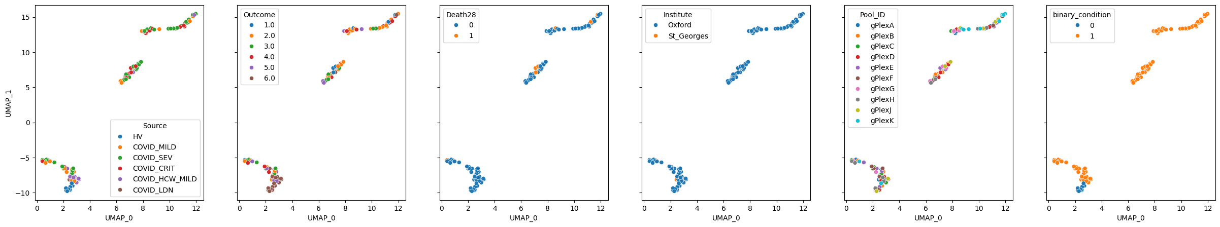
While it is not clear why we see 3 clusters, healthy volunteers are clearly grouped together
Since binary_condition was specified as a label during training, we can predict this label with PaSCient’s classifier:
pascient_prediction = pascient.predict("binary_condition")
pascient_prediction
| prob_0 | prob_1 | binary_condition_pred | |
|---|---|---|---|
| S00109-Ja001E-PBCa | 0.000044 | 0.999956 | 1 |
| S00112-Ja003E-PBCa | 0.003916 | 0.996083 | 1 |
| S00005-Ja005E-PBCa | 0.000296 | 0.999704 | 1 |
| S00061-Ja003E-PBCa | 0.000095 | 0.999905 | 1 |
| S00056-Ja003E-PBCa | 0.002233 | 0.997767 | 1 |
| ... | ... | ... | ... |
| S00076-Ja001E-PBCa | 0.002672 | 0.997328 | 1 |
| S00072-Ja001E-PBCa | 0.000039 | 0.999961 | 1 |
| S00065-Ja003E-PBCa | 0.000191 | 0.999809 | 1 |
| S00048-Ja003E-PBCa | 0.000182 | 0.999818 | 1 |
| G05112-Ja005E-PBCa | 0.000029 | 0.999971 | 1 |
101 rows × 3 columns
y_true = metadata.loc[pascient_prediction.index, "binary_condition"]
print(classification_report(y_true, pascient_prediction["binary_condition_pred"]))
              precision    recall  f1-score   support

           0       1.00      1.00      1.00        10
           1       1.00      1.00      1.00        91

    accuracy                           1.00       101
   macro avg       1.00      1.00      1.00       101
weighted avg       1.00      1.00      1.00       101
Now let’s challenge paSCient with a more complex task of multilabel classification of disease severities:
metadata["Source"].value_counts()
Source
COVID_SEV         41
COVID_MILD        18
COVID_CRIT        18
COVID_HCW_MILD    12
HV                10
COVID_LDN          2
Name: count, dtype: int64
pascient.fine_tune("Source", tasks="classification")
┏━━━┳━━━━━━━━━━━━━━━━━━━━━━━━━━━━━┳━━━━━━━━━━━━━━━━━━━━━━━━━┳━━━━━━━━┳━━━━━━━┳━━━━━━━┓
┃   ┃ Name                        ┃ Type                    ┃ Params ┃ Mode  ┃ FLOPs ┃
┡━━━╇━━━━━━━━━━━━━━━━━━━━━━━━━━━━━╇━━━━━━━━━━━━━━━━━━━━━━━━━╇━━━━━━━━╇━━━━━━━╇━━━━━━━┩
│ 0 │ gene2cell_encoder           │ BasicMLP                │  3.1 M │ train │     0 │
│ 1 │ cell2patient_aggregation    │ NonLinearAttnAggregator │  1.1 M │ train │     0 │
│ 2 │ patient_encoder             │ BasicMLP                │  787 K │ train │     0 │
│ 3 │ cell2cell_encoder           │ CellToCellIdentity      │      0 │ train │     0 │
│ 4 │ sample_prediction_loss_func │ CrossEntropyLossViews   │      0 │ train │     0 │
│ 5 │ patient_predictor           │ BasicMLP                │  3.1 K │ train │     0 │
└───┴─────────────────────────────┴─────────────────────────┴────────┴───────┴───────┘
Trainable params: 4.9 M
Non-trainable params: 0
Total params: 4.9 M
Total estimated model params size (MB): 19
Modules in train mode: 20
Modules in eval mode: 0
Total FLOPs: 0
/home/icb/vladimir.shitov/software/miniconda3/envs/patpy/lib/python3.13/site-packages/rich/live.py:260:
UserWarning: install "ipywidgets" for Jupyter support
  warnings.warn('install "ipywidgets" for Jupyter support')
/home/icb/vladimir.shitov/software/miniconda3/envs/patpy/lib/python3.13/site-packages/lightning/pytorch/utilities/_
pytree.py:21: `isinstance(treespec, LeafSpec)` is deprecated, use `isinstance(treespec, TreeSpec) and
treespec.is_leaf()` instead.
/home/icb/vladimir.shitov/software/miniconda3/envs/patpy/lib/python3.13/site-packages/lightning/pytorch/trainer/con
nectors/data_connector.py:434: The 'val_dataloader' does not have many workers which may be a bottleneck. Consider
increasing the value of the `num_workers` argument` to `num_workers=7` in the `DataLoader` to improve performance.
/home/icb/vladimir.shitov/software/miniconda3/envs/patpy/lib/python3.13/site-packages/lightning/pytorch/trainer/con
nectors/data_connector.py:434: The 'train_dataloader' does not have many workers which may be a bottleneck.
Consider increasing the value of the `num_workers` argument` to `num_workers=7` in the `DataLoader` to improve
performance.
pascient_source_prediction = pascient.predict("Source")
pascient_source_prediction
| prob_COVID_CRIT | prob_COVID_HCW_MILD | prob_COVID_LDN | prob_COVID_MILD | prob_COVID_SEV | prob_HV | Source_pred | |
|---|---|---|---|---|---|---|---|
| S00109-Ja001E-PBCa | 0.394535 | 0.025477 | 0.025743 | 0.144956 | 0.409188 | 0.000101 | COVID_SEV |
| S00112-Ja003E-PBCa | 0.063328 | 0.267164 | 0.217097 | 0.295604 | 0.150487 | 0.006321 | COVID_MILD |
| S00005-Ja005E-PBCa | 0.880595 | 0.003001 | 0.008579 | 0.024722 | 0.083051 | 0.000052 | COVID_CRIT |
| S00061-Ja003E-PBCa | 0.388946 | 0.029524 | 0.029042 | 0.148687 | 0.403622 | 0.000178 | COVID_SEV |
| S00056-Ja003E-PBCa | 0.210393 | 0.132618 | 0.112567 | 0.244251 | 0.297248 | 0.002924 | COVID_SEV |
| ... | ... | ... | ... | ... | ... | ... | ... |
| S00076-Ja001E-PBCa | 0.125680 | 0.192639 | 0.150116 | 0.281483 | 0.246566 | 0.003515 | COVID_MILD |
| S00072-Ja001E-PBCa | 0.361417 | 0.029526 | 0.027950 | 0.170613 | 0.410370 | 0.000123 | COVID_SEV |
| S00065-Ja003E-PBCa | 0.398539 | 0.032703 | 0.032377 | 0.143577 | 0.392591 | 0.000213 | COVID_CRIT |
| S00048-Ja003E-PBCa | 0.378879 | 0.033592 | 0.032130 | 0.151074 | 0.404112 | 0.000212 | COVID_SEV |
| G05112-Ja005E-PBCa | 0.287130 | 0.048738 | 0.032903 | 0.213581 | 0.417497 | 0.000151 | COVID_SEV |
101 rows × 7 columns
source_true = metadata.loc[pascient_source_prediction.index, "Source"]
print(classification_report(source_true, pascient_source_prediction["Source_pred"]))
                precision    recall  f1-score   support

    COVID_CRIT       0.68      0.72      0.70        18
COVID_HCW_MILD       0.59      0.83      0.69        12
     COVID_LDN       0.00      0.00      0.00         2
    COVID_MILD       0.60      0.50      0.55        18
     COVID_SEV       0.72      0.71      0.72        41
            HV       1.00      1.00      1.00        10

      accuracy                           0.70       101
     macro avg       0.60      0.63      0.61       101
  weighted avg       0.69      0.70      0.69       101
Not bad! PaSCient achieves macro F1 score of 0.61, the best we’ve seen so far
The sample embeddings has changed after fine-tuning as the entire model was retrained. Let’s visualise them:
pascient_distances = pascient.calculate_distance_matrix()
pascient.embed("UMAP")
pascient.plot_embedding(method="UMAP", metadata_cols=samples_metadata_cols, continuous_palette="tab10");
Cell importance#
PaSCient can compute per-cell importance scores to identify which cells contribute most to sample-level representations.
Note: By default,
get_cell_importance()uses Integrated Gradients (IG) from the PaSCient paper when captum is installed, and falls back to cosine similarity between cell and sample embeddings otherwise.
cell_importance = pascient.get_cell_importance(target=1)
importance_scores = cell_importance.iloc[:, 0]
print(f"Importance scores: min={importance_scores.min():.4f}, max={importance_scores.max():.4f}, mean={importance_scores.mean():.4f}")
Importance scores: min=0.0000, max=0.0415, mean=0.0000
Cell importance by disease severity and cell type#
Visualize the distribution of cell importance scores. Since most scores are near zero with a long tail of important cells, we use strip plots with log-scaled y-axis for better visibility.
import seaborn as sns

# Build dataframe with importance scores and metadata
cell_imp_df = pd.DataFrame({
    "importance": importance_scores,
    "Source": adata.obs["Source"].values,
    "cell_type": adata.obs[cell_type_key].values,
}, index=adata.obs_names)

severity_order = ["HV", "COVID_HCW_MILD", "COVID_MILD", "COVID_LDN", "COVID_SEV", "COVID_CRIT"]

fig, axes = plt.subplots(1, 2, figsize=(16, 5))

# Filter to nonzero for log-scale
nonzero = cell_imp_df[cell_imp_df["importance"] > 0]

# By disease severity
ax = axes[0]
sns.boxplot(data=nonzero, x="Source", y="importance", order=severity_order, ax=ax)
ax.set_yscale("log")
ax.set_xlabel("Disease severity")
ax.set_ylabel("Cell importance")
ax.set_title("Cell importance by disease severity")
ax.tick_params(axis="x", rotation=45)

# By cell type
ax = axes[1]
sns.boxplot(data=nonzero, x="cell_type", y="importance", ax=ax)
ax.set_yscale("log")
ax.set_xlabel("Cell type")
ax.set_ylabel("Cell importance")
ax.set_title("Cell importance by cell type")
ax.tick_params(axis="x", rotation=45)

plt.tight_layout()
plt.show()
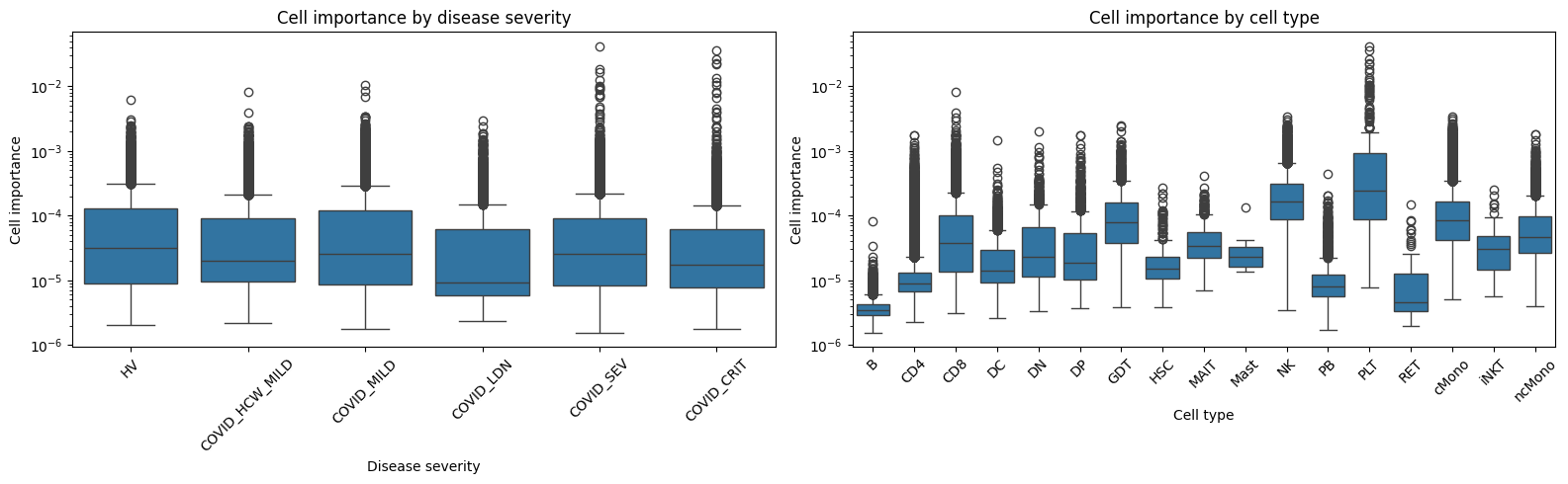
The distributions per disease severity look quite similar, but maximum cell importances seem larger for more severe COVID stages
Summary statistics#
Descriptive statistics of cell importance scores grouped by disease severity and cell type.
print("=== Cell importance by disease severity ===")
cell_imp_df.groupby("Source")["importance"].describe().loc[severity_order].round(6)
=== Cell importance by disease severity ===
| count | mean | std | min | 25% | 50% | 75% | max | |
|---|---|---|---|---|---|---|---|---|
| Source | ||||||||
| HV | 87204.0 | 0.000018 | 0.000088 | 0.0 | 0.0 | 0.0 | 0.000000 | 0.006155 |
| COVID_HCW_MILD | 84359.0 | 0.000018 | 0.000088 | 0.0 | 0.0 | 0.0 | 0.000000 | 0.008232 |
| COVID_MILD | 107376.0 | 0.000027 | 0.000121 | 0.0 | 0.0 | 0.0 | 0.000003 | 0.010584 |
| COVID_LDN | 14832.0 | 0.000017 | 0.000093 | 0.0 | 0.0 | 0.0 | 0.000000 | 0.002996 |
| COVID_SEV | 230343.0 | 0.000021 | 0.000139 | 0.0 | 0.0 | 0.0 | 0.000004 | 0.041486 |
| COVID_CRIT | 87620.0 | 0.000018 | 0.000210 | 0.0 | 0.0 | 0.0 | 0.000007 | 0.035924 |
print("=== Cell importance by cell type (sorted by max) ===")
cell_imp_df.groupby("cell_type")["importance"].describe().round(6).sort_values("max", ascending=False)
=== Cell importance by cell type (sorted by max) ===
| count | mean | std | min | 25% | 50% | 75% | max | |
|---|---|---|---|---|---|---|---|---|
| cell_type | ||||||||
| PLT | 920.0 | 0.000544 | 0.002747 | 0.0 | 0.0 | 0.0 | 0.000052 | 0.041486 |
| CD8 | 87562.0 | 0.000020 | 0.000078 | 0.0 | 0.0 | 0.0 | 0.000000 | 0.008232 |
| cMono | 152220.0 | 0.000035 | 0.000105 | 0.0 | 0.0 | 0.0 | 0.000015 | 0.003444 |
| NK | 57648.0 | 0.000058 | 0.000161 | 0.0 | 0.0 | 0.0 | 0.000000 | 0.003357 |
| GDT | 7935.0 | 0.000033 | 0.000109 | 0.0 | 0.0 | 0.0 | 0.000000 | 0.002455 |
| DN | 3426.0 | 0.000015 | 0.000066 | 0.0 | 0.0 | 0.0 | 0.000000 | 0.002018 |
| ncMono | 21281.0 | 0.000019 | 0.000062 | 0.0 | 0.0 | 0.0 | 0.000000 | 0.001800 |
| DP | 5354.0 | 0.000014 | 0.000064 | 0.0 | 0.0 | 0.0 | 0.000000 | 0.001764 |
| CD4 | 218353.0 | 0.000004 | 0.000017 | 0.0 | 0.0 | 0.0 | 0.000000 | 0.001737 |
| DC | 7287.0 | 0.000007 | 0.000027 | 0.0 | 0.0 | 0.0 | 0.000000 | 0.001444 |
| PB | 6945.0 | 0.000004 | 0.000012 | 0.0 | 0.0 | 0.0 | 0.000004 | 0.000440 |
| MAIT | 3977.0 | 0.000009 | 0.000024 | 0.0 | 0.0 | 0.0 | 0.000000 | 0.000407 |
| HSC | 1124.0 | 0.000007 | 0.000021 | 0.0 | 0.0 | 0.0 | 0.000009 | 0.000269 |
| iNKT | 360.0 | 0.000010 | 0.000027 | 0.0 | 0.0 | 0.0 | 0.000000 | 0.000253 |
| RET | 197.0 | 0.000005 | 0.000016 | 0.0 | 0.0 | 0.0 | 0.000003 | 0.000151 |
| Mast | 42.0 | 0.000008 | 0.000022 | 0.0 | 0.0 | 0.0 | 0.000000 | 0.000133 |
| B | 37103.0 | 0.000001 | 0.000002 | 0.0 | 0.0 | 0.0 | 0.000002 | 0.000080 |
In this tutorial you learned how to run supervised sample-level methods, evaluate and visualise the results with patpy