Synthetic data generation

In this notebook, we will generate synthetic data with perturbation of cell type abundance and/or gene expression. It will help us to understand what different patient representation method pay attention to. We will use the PBMC3k dataset for this purpose. It has peripheral blood mononuclear cells from 3k cells of a healthy donor. We will simulate synthetic donors perturbing hallmarks of severe COVID-19 described in the COMBAT study.

Perturbations can happen in two ways:

• Composition shift - cells have a similar expression profile but samples have different cell type abundance depending on the severity of the disease.

• Expression shift - samples have a similar cell type abundance but different expression profile depending on the severity of the disease.

• Jointly - both composition and expression are perturbed depending on the severity of the disease

Here, we’ll simulate all 3 cases.

import warnings

import scanpy as sc
import matplotlib.pyplot as plt
import numpy as np
import pandas as pd

from datasets.synthetic import simulate_data, covid_19_hallmarks, process_adata

warnings.filterwarnings("ignore")

Data preparation

The data can be loaded from the Scanpy package. We will take cell types from the processed data, but will use the original data to work with raw gene expression.

processed_adata = sc.datasets.pbmc3k_processed()
adata = sc.datasets.pbmc3k()
adata = adata[processed_adata.obs_names]

cell_type_key = "louvain"
adata.obs[cell_type_key] = processed_adata.obs[cell_type_key]

adata.obsp = processed_adata.obsp  # Copy distances to further use nearest neighbors in the simulation

Some of the hallmarks for COVID-19 can be imported from the patpy.datasets.synthetic module. They contain cell types and genes that are affected by the disease.

Defining perturbations

severe_covid_19_abundance_hallmarks, severe_covid_19_expression_hallmarks = covid_19_hallmarks()

Abundance hallmarks are fold changes for cell type proportions. For example, CD14+ Monocytes were found to roughly double in proportion in patients with severe COVID-19 while CD8 T cells were found to decrease to 50% of their original level. This is reflected in the dictionary below with fold changes 2 and 0.5 for CD14+ Monocytes and CD8 T cells respectively:

severe_covid_19_abundance_hallmarks

{'FCGR3A+ Monocytes': 0.4,
 'Dendritic cells': 0.2,
 'CD14+ Monocytes': 2,
 'CD8 T cells': 0.5,
 'NK cells': 4}

Expression hallmarks are fold changes for gene expression. We are using only a small subset of genes that are affected by the disease. For more details on where these numbers come from, check out the covid_19_hallmarks function in the source code

severe_covid_19_expression_hallmarks

{'CD4 T cells': {'IFITM1': 0.5, 'ID3': 26.666666666666668, 'TUBA1B': 0.55},
 'CD8 T cells': {'MT-CO1': 5.5, 'GNLY': 0.25},
 'NK cells': {'S1PR1': 15.866666666666667},
 'B cells': {'TXNIP': 0.42},
 'CD14+ Monocytes': {'S100A8': 7.666666666666666,
  'HLA-DQA1': 0.125,
  'CLU': 220.85651708616052,
  'FAM20A': 206.06641683730044,
  'PIM3': 13.333333333333334,
  'CYP19A1': 228.64500534107583,
  'PIM1': 46.42936337579328,
  'CDKN2D': 6.666666666666667,
  'CDIP1': 0.2871745887492587,
  'CACNA2D3': 0.0625,
  'ZNF217': 0.6597539553864471,
  'ZNF703': 0.125,
  'ADAMTS5': 0.03125,
  'HLA-DQA2': 0.03589682359365735}}

The dictionaries above define maximum fold changes (i.e. at the most severe point). We will gradually increase the perturbation strength to simulate a continuous trajectory from healthy to severe COVID-19.

Not all perturbed genes are in the list of highly variable genes. Let’s add them to the list of genes to keep to further use them in the analysis.

perturbed_genes = []

for cell_type, degs in severe_covid_19_expression_hallmarks.items():
    perturbed_genes.extend(degs.keys())

genes_to_keep = list(set(processed_adata.var_names.tolist() + perturbed_genes))

adata.raw = adata
adata = adata[:, genes_to_keep]

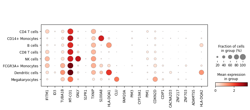
sc.pl.dotplot(adata, perturbed_genes, groupby=cell_type_key, log=True)

Not all hallmarks genes are highly expressed in the PBMC3k data, so let’s add some random genes as well. We’ll perturb them in B cells as abundant class but not very well covered in the dictionary above.

# To select highly expressed genes
sc.pp.calculate_qc_metrics(adata, inplace=True)

n_affected_genes = 16
affected_cell_type = "B cells"

expressed_genes = adata.var_names[adata.var["pct_dropout_by_counts"] < 80]

# Select some genes to decrease their expression with the perturbation strength
downregulated_genes = np.random.choice(expressed_genes, size=n_affected_genes // 2)

# Select some genes (that are not downregulated) to increase their expression with the perturbation strength
upregulated_genes = np.random.choice(
    expressed_genes[~np.isin(expressed_genes, downregulated_genes)], size=n_affected_genes // 2
)

for gene in downregulated_genes:
    severe_covid_19_expression_hallmarks[affected_cell_type][gene] = np.random.uniform(0.01, 0.2)

for gene in upregulated_genes:
    severe_covid_19_expression_hallmarks[affected_cell_type][gene] = (
        np.random.uniform(2, 128) / 0.3
    )  # Considering dropout, let's make effect size even more than expected

Data simulation

Let’s now simulate 3 scenarios with different perturbation types:

• Composition shift - cells have a similar expression profile but samples have different cell type abundance depending on the severity of the disease defined by the perturbation strength.

• Expression shift - samples have a similar cell type abundance but different expression profile depending on the severity of the disease.

• Jointly - both composition and expression are perturbed depending on the severity of the disease

%%time

adata.obs["perturbation_strength"] = 0

n_samples = 41

composition_perturbed_adatas = []
expression_perturbed_adatas = []
jointly_perturbed_adatas = []

for perturbation_strength in np.linspace(0, 1, n_samples):
    print(f"Simulating data with perturbation strength {perturbation_strength}")
    perturbed_adata = adata.copy()
    perturbed_adata.obs["perturbation_strength"] = perturbation_strength

    print("Simulating composition perturbation")
    composition_perturbed_adatas.append(
        simulate_data(
            perturbed_adata.copy(),
            cell_type_key,
            abundance_perturbation=severe_covid_19_abundance_hallmarks,
            gene_perturbation=None,
            perturbation_strength=perturbation_strength,
            expression_noise_scale=1,
        )
    )
    print("Simulating expression perturbation")
    expression_perturbed_adatas.append(
        simulate_data(
            perturbed_adata.copy(),
            cell_type_key,
            abundance_perturbation=None,
            gene_perturbation=severe_covid_19_expression_hallmarks,
            perturbation_strength=perturbation_strength,
            expression_noise_scale=1,
        )
    )
    print("Simulating jointly perturbation")
    jointly_perturbed_adatas.append(
        simulate_data(
            perturbed_adata.copy(),
            cell_type_key,
            abundance_perturbation=severe_covid_19_abundance_hallmarks,
            gene_perturbation=severe_covid_19_expression_hallmarks,
            perturbation_strength=perturbation_strength,
            expression_noise_scale=1,
        )
    )
    print("-" * 100, end="\n\n")

composition_perturbed_adata = sc.concat(composition_perturbed_adatas, axis=0)
expression_perturbed_adata = sc.concat(expression_perturbed_adatas, axis=0)
jointly_perturbed_adata = sc.concat(jointly_perturbed_adatas, axis=0)

composition_perturbed_adata.obs["perturbation_type"] = "composition"
expression_perturbed_adata.obs["perturbation_type"] = "expression"
jointly_perturbed_adata.obs["perturbation_type"] = "joint"

Simulating data with perturbation strength 0.0
Simulating composition perturbation
Simulating expression perturbation
Simulating jointly perturbation
----------------------------------------------------------------------------------------------------

Simulating data with perturbation strength 0.1
Simulating composition perturbation
Simulating expression perturbation
Simulating jointly perturbation
----------------------------------------------------------------------------------------------------

Simulating data with perturbation strength 0.2
Simulating composition perturbation
Simulating expression perturbation
Simulating jointly perturbation
----------------------------------------------------------------------------------------------------

Simulating data with perturbation strength 0.30000000000000004
Simulating composition perturbation
Simulating expression perturbation
Simulating jointly perturbation
----------------------------------------------------------------------------------------------------

Simulating data with perturbation strength 0.4
Simulating composition perturbation
Simulating expression perturbation
Simulating jointly perturbation
----------------------------------------------------------------------------------------------------

Simulating data with perturbation strength 0.5
Simulating composition perturbation
Simulating expression perturbation
Simulating jointly perturbation
----------------------------------------------------------------------------------------------------

Simulating data with perturbation strength 0.6000000000000001
Simulating composition perturbation
Simulating expression perturbation
Simulating jointly perturbation
----------------------------------------------------------------------------------------------------

Simulating data with perturbation strength 0.7000000000000001
Simulating composition perturbation
Simulating expression perturbation
Simulating jointly perturbation
----------------------------------------------------------------------------------------------------

Simulating data with perturbation strength 0.8
Simulating composition perturbation
Simulating expression perturbation
Simulating jointly perturbation
----------------------------------------------------------------------------------------------------

Simulating data with perturbation strength 0.9
Simulating composition perturbation
Simulating expression perturbation
Simulating jointly perturbation
----------------------------------------------------------------------------------------------------

Simulating data with perturbation strength 1.0
Simulating composition perturbation
Simulating expression perturbation
Simulating jointly perturbation
----------------------------------------------------------------------------------------------------

CPU times: user 19.9 s, sys: 1.19 s, total: 21.1 s
Wall time: 21.9 s

Quickly process the data to make it ready for the analysis. The function process_adata will normalize the data, do log transformation, scale the expression, calculate PCA, UMAP and neighbors following the standard scanpy pipeline.

As we have a lot of samples, the processing will take some time and can require a lot of memory. If your machine struggles with it, you can decrease the number of samples or work with different perturbations one by one.

%%time

print("Processing composition perturbed data")
composition_perturbed_adata = process_adata(composition_perturbed_adata, verbose=True)

print("\nProcessing expression perturbed data")
expression_perturbed_adata = process_adata(expression_perturbed_adata, verbose=True)

print("\nProcessing jointly perturbed data")
jointly_perturbed_adata = process_adata(jointly_perturbed_adata, verbose=True)

Processing composition perturbed data
Calculating QC metrics...
Normalizing...
Log transforming...
Scaling...
PCA...
Building neighbors graph...
UMAP...

Processing expression perturbed data
Calculating QC metrics...
Normalizing...
Log transforming...
Scaling...
PCA...
Building neighbors graph...
UMAP...

Processing jointly perturbed data
Calculating QC metrics...
Normalizing...
Log transforming...
Scaling...
PCA...
Building neighbors graph...
UMAP...
CPU times: user 6min 45s, sys: 23.2 s, total: 7min 8s
Wall time: 2min 43s

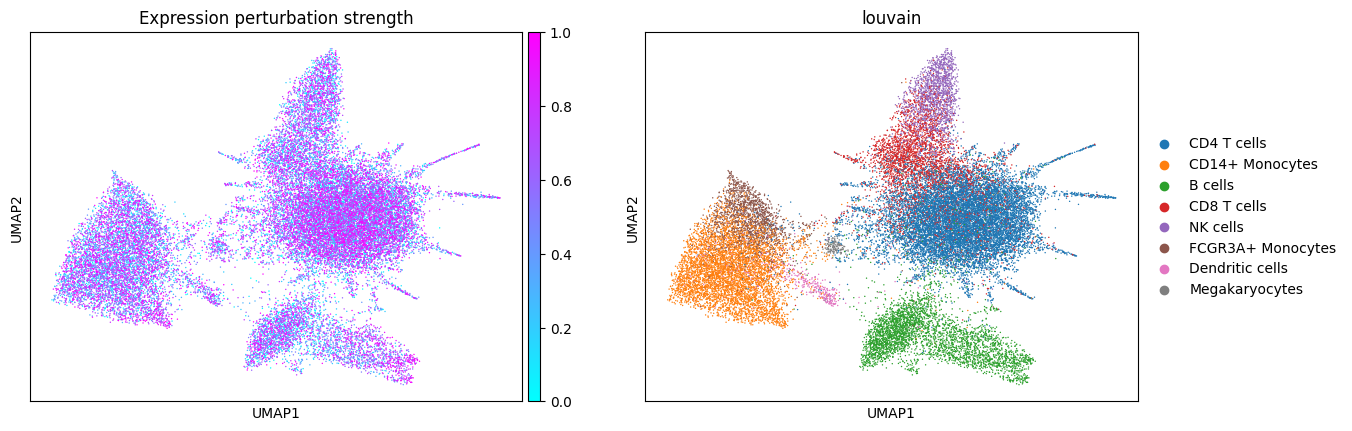
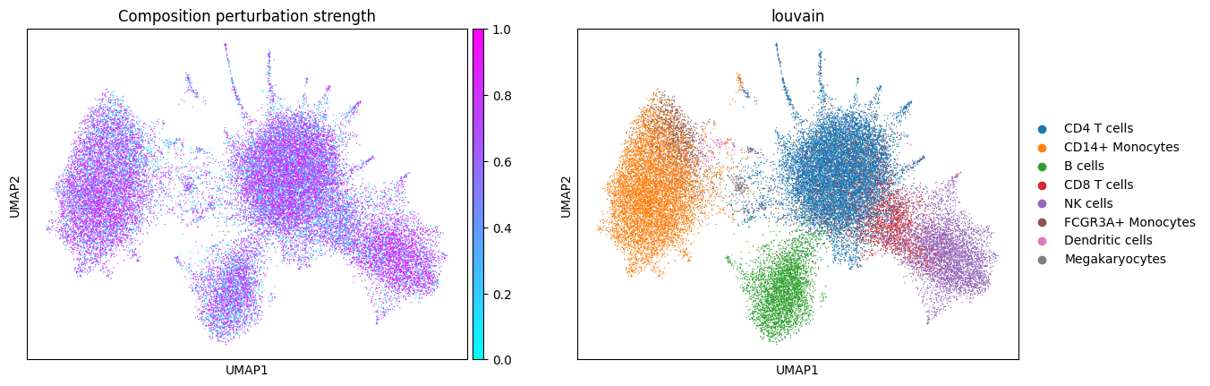
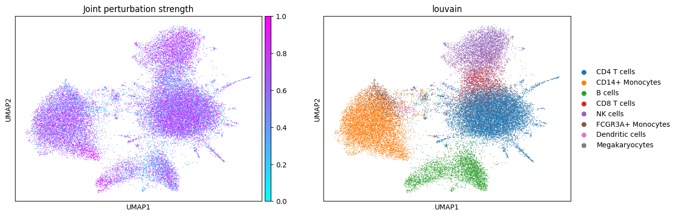
Let’s see what the simulated data looks like! Note the presence of disease-specific cell states for CD14+ Monocytes and B cells when expression is perturbed (groups of cells with purple color and no blue in between). The composition shift is easier to spot by looking at NK cells: there are more of them in the composition perturbed data.

Analysis of the simulated data

First, let’s see what the data embedding looks like for different perturbation types.

cols_to_plot = ["perturbation_strength", cell_type_key]

sc.pl.umap(expression_perturbed_adata, color=cols_to_plot, title="Expression perturbation strength", cmap="cool")
sc.pl.umap(composition_perturbed_adata, color=cols_to_plot, title="Composition perturbation strength", cmap="cool")
sc.pl.umap(jointly_perturbed_adata, color=cols_to_plot, title="Joint perturbation strength", cmap="cool")

WARNING: The title list is shorter than the number of panels. Using 'color' value instead for some plots.
WARNING: The title list is shorter than the number of panels. Using 'color' value instead for some plots.
WARNING: The title list is shorter than the number of panels. Using 'color' value instead for some plots.

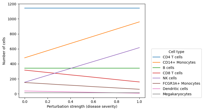
In composition perturbation cell type abundances change linearly with the perturbation strength:

pd.crosstab(
    composition_perturbed_adata.obs["perturbation_strength"], composition_perturbed_adata.obs[cell_type_key]
).plot.line()
plt.xlabel("Perturbation strength (disease severity)")
plt.ylabel("Number of cells")
plt.legend(loc=(1.05, 0), title="Cell type")

<matplotlib.legend.Legend at 0x2a8f569b0>

We can also see how genes are perturbed in the expression perturbation:

sc.pl.umap(
    expression_perturbed_adata,
    color=["perturbation_strength", "total_counts", cell_type_key] + perturbed_genes,
    cmap="Reds",
)

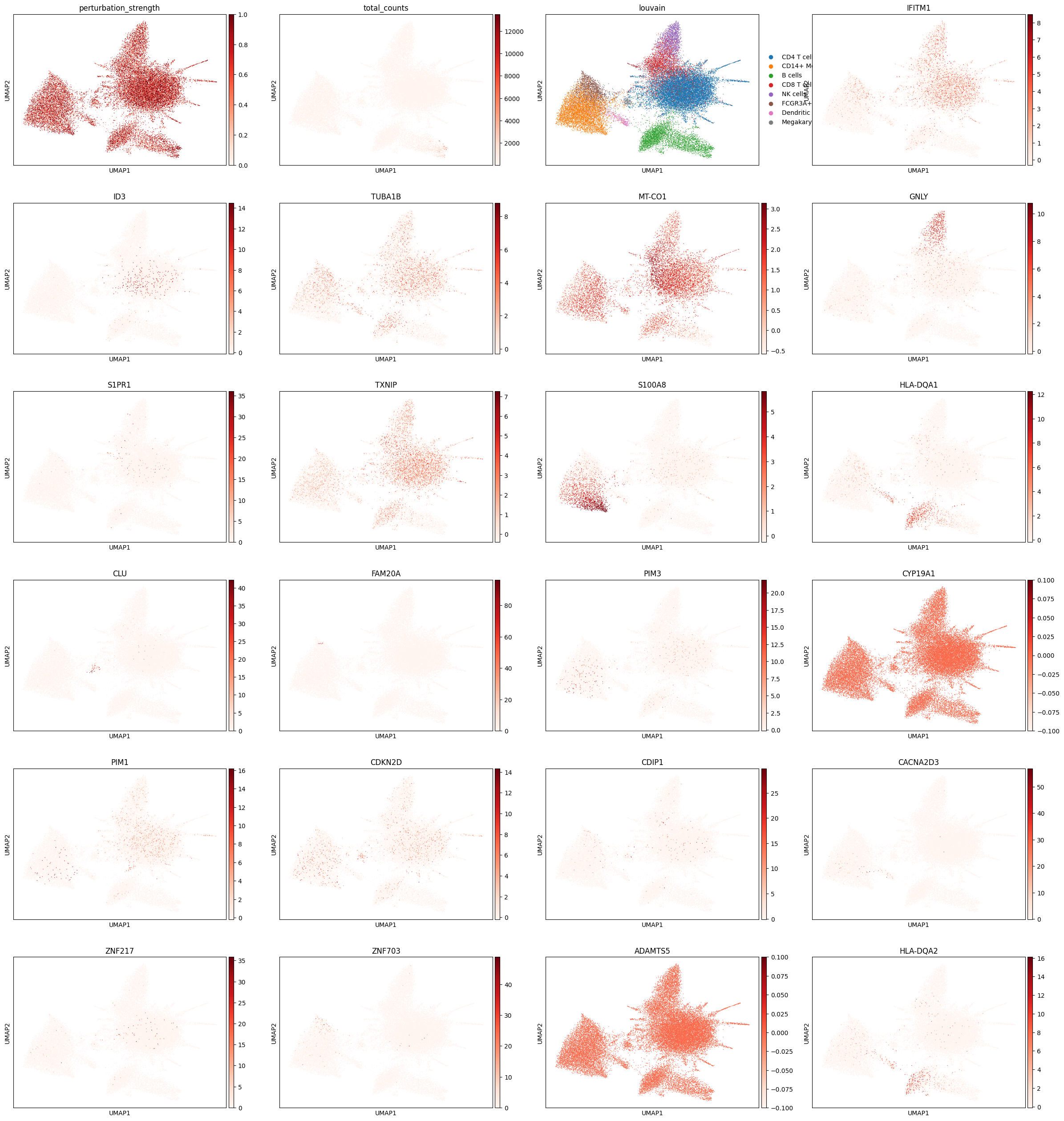
The jointly perturbed data has a combination of the composition and expression perturbations

Patient representation analysis

Let’s explore how simple patient representation methods work on the simulated data. We will start with pseudobulking and composition differences. Intuitively, pseudobulking should capture both composition and expression shift effects, while composition differences should only capture composition shift.

import patpy

composition_perturbed_adata.obs["sample_key"] = "sample_" + composition_perturbed_adata.obs[
    "perturbation_strength"
].astype(str)
expression_perturbed_adata.obs["sample_key"] = "sample_" + expression_perturbed_adata.obs[
    "perturbation_strength"
].astype(str)
jointly_perturbed_adata.obs["sample_key"] = "sample_" + jointly_perturbed_adata.obs["perturbation_strength"].astype(str)

fig, axes = plt.subplots(ncols=2, nrows=3, figsize=(10, 15))

for perturbed_adata, ax in zip(
    [composition_perturbed_adata, expression_perturbed_adata, jointly_perturbed_adata], axes, strict=False
):
    pseudobulk = patpy.tl.Pseudobulk("sample_key", cell_type_key)
    pseudobulk.prepare_anndata(perturbed_adata)
    pseudobulk.calculate_distance_matrix()
    pseudobulk.plot_embedding("MDS", metadata_cols=["perturbation_strength"], axes=ax[0])
    ax[0].set_title(
        "Pseudobulk representation of " + perturbed_adata.obs["perturbation_type"][0] + " perturbed data", fontsize=10
    )
    ax[0].get_legend().remove()
    ax[0].set_xticks([])
    ax[0].set_yticks([])

    composition = patpy.tl.CellGroupComposition("sample_key", cell_type_key)
    composition.prepare_anndata(perturbed_adata)
    composition.calculate_distance_matrix()
    composition.plot_embedding("MDS", metadata_cols=["perturbation_strength"], axes=ax[1])
    ax[1].set_title(
        "Composition representation of " + perturbed_adata.obs["perturbation_type"][0] + " perturbed data", fontsize=10
    )
    ax[1].set_ylabel("")
    ax[1].set_xticks([])
    ax[1].set_yticks([])

    if perturbed_adata is not jointly_perturbed_adata:  # Plot legen only on the last frame
        ax[1].get_legend().remove()

0 samples removed: 
0 cell types removed: 
0 samples removed: 
0 cell types removed: 
0 samples removed: 
0 cell types removed: 
0 samples removed: 
0 cell types removed:
0 samples removed: 
0 cell types removed: 
0 samples removed: 
0 cell types removed:

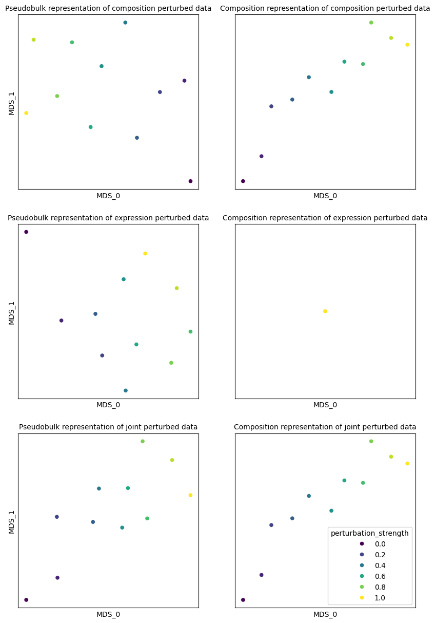
As we can see, pseudobulking captures both composition and expression shift effects, while composition differences only capture composition shift. Joint perturbation is captured well by both methods. We can evaluate it by predicting perturbation strength (disease severity) from the representation:

pseudobulk.evaluate_representation(target="perturbation_strength", task="regression")

{'score': 0.9868667917448407,
 'metric': 'spearman_r',
 'n_unique': 40,
 'n_observations': 40,
 'method': 'knn'}

composition.evaluate_representation(target="perturbation_strength", task="regression")

{'score': 0.998874296435272,
 'metric': 'spearman_r',
 'n_unique': 40,
 'n_observations': 40,
 'method': 'knn'}

expression_perturbed_adata.write("../../docs/notebooks/data/synthetic_expression_perturbed.h5ad")
composition_perturbed_adata.write("../../docs/notebooks/data/synthetic_composition_perturbed.h5ad")
jointly_perturbed_adata.write("../../docs/notebooks/data/synthetic_jointly_perturbed.h5ad")